
In this article we are going to consider our first intraday trading strategy. It will be using a classic trading idea, that of "trading pairs". In this instance we are going to be making use of two Exchange Traded Funds (ETFs), SPY and IWM, which are traded on the New York Stock Exchange (NYSE) and attempt to represent the US stock market indices, the S&P500 and the Russell 2000, respectively.
The strategy broadly creates a "spread" between the pair of ETFs by longing one and shorting an amount of the other. The ratio of long to short can be defined in many ways such as utilising statistical cointegrating time series techniques. In this scenario we are going to calculate a hedge ratio between SPY and IWM via a rolling linear regression. This will then allow us to create a "spread" between SPY and IWM which is normalised to a z-score. The trading signals will be generated when the z-score exceeds certain thresholds under the belief that the spread will revert to the mean.
The rationale for the strategy is that SPY and IWM are approximately characterising the same situation, that of the economics of a group of large-cap and small-cap US corporations. The premise is that if one takes the spread of the prices then it should be mean-reverting, since while "local" (in time) events may effect either the S&P500 or the Russell 2000 indices separately (such as small-cap/large-cap differences, rebalancing dates or block trades), the long-term price series of the two will likely be cointegrated.
The Strategy
The strategy is carried out in the following steps:
- Data - 1-minute bars of SPY and IWM are obtained from April 2007 through to February 2014.
- Processing - The data are correctly aligned and missing bars are mutually discarded.
- Spread - The hedge ratio between the two ETFs is calculated by taking a rolling linear regression. This is defined as the β regression coefficient using a lookback window which shifts forward by 1 bar and recalculates the regression coefficients. Thus the hedge ratio βi, for bar bi is calculated across points bi−1−k to bi−1 for a lookback of k bars.
- Z-Score - The standard score of the spread is calculated in the usual manner. This means subtracting the (sample) mean of the spread and dividing by the (sample) standard deviation of the spread. The rationale for this is to make threshold parameters more straightforward to interpet since the z-score is a dimensionless quantity. I have deliberately introduced a lookahead bias into the calculations in order to show how subtle it can be. Try and look out for it!
- Trades - Long signals are generated when the negative z-score drops below a pre-determined (or post-optimised) threshold, while short signals are the converse of this. Exit signals are generated when the absolute z-score drops below an additional threshold. For this strategy I have (somewhat arbitrarily) picked an absolute entry threshold of |z|=2 and an exit threshold of |z|=1. Assuming mean reverting behaviour in the spread, this will hopefully capture that relationship and provide positive performance.
Perhaps the best way to understand the strategy in depth is to actually implement it. The following section describes a full Python code (single file) for implementing this mean-reverting strategy. I have liberally commented the code in order to aid understanding.
Python Implementation
As with all of the Python/pandas tutorials it is necessary to have setup a Python research environment as described in this tutorial. Once setup, the first task is to import the necessary Python libraries. For this backtest matplotlib and pandas are required.
The specific library versions that I am using are as follows:
- Python - 2.7.3
- NumPy - 1.8.0
- pandas - 0.12.0
- matplotlib - 1.1.0
Let's go ahead and import the librararies:
python
# mr_spy_iwm.py
import matplotlib.pyplot as plt
import numpy as np
import os, os.path
import pandas as pd
The following function create_pairs_dataframe imports two CSV files containing the intraday bars of two symbols. In our case this will be SPY and IWM. It then creates a separate dataframe pairs, which uses the indexes of both original files. Since their timestamps are likely to be different due to missed trades and errors, this guarantees that we will have matching data. This is one of the main benefits of using a data analyis library like pandas. The "boilerplate" code is handled for us in a very efficient manner.
            python

            # mr_spy_iwm.py

def create_pairs_dataframe(datadir, symbols):
    """Creates a pandas DataFrame containing the closing price
    of a pair of symbols based on CSV files containing a datetime
    stamp and OHLCV data."""

    # Open the individual CSV files and read into pandas DataFrames
    print "Importing CSV data..."
    sym1 = pd.io.parsers.read_csv(os.path.join(datadir, '%s.csv' % symbols[0]),
                                  header=0, index_col=0,
                                  names=['datetime','open','high','low','close','volume','na'])
    sym2 = pd.io.parsers.read_csv(os.path.join(datadir, '%s.csv' % symbols[1]),
                                  header=0, index_col=0,
                                  names=['datetime','open','high','low','close','volume','na'])

    # Create a pandas DataFrame with the close prices of each symbol
    # correctly aligned and dropping missing entries
    print "Constructing dual matrix for %s and %s..." % symbols
    pairs = pd.DataFrame(index=sym1.index)
    pairs['%s_close' % symbols[0].lower()] = sym1['close']
    pairs['%s_close' % symbols[1].lower()] = sym2['close']
    pairs = pairs.dropna()
    return pairs
The next step is to carry out the rolling linear regression between SPY and IWM. In this instance IWM is the predictor ('x') and SPY is the response ('y'). I have set a default lookback window of 100 bars. As discussed above this is a parameter of the strategy. In order for the strategy to be considered robust we ideally want to see a returns profile (or other measure of performance) as a convex function of lookback period. Thus at a later stage in the code we will carry out a sensitivity analysis by varying the lookback period over a range.
Once the rolling beta coefficient is calculated in the linear regression model for SPY-IWM, we add it to the pairs DataFrame and drop the empty rows. This constitutes the first set of bars equal to the size of the lookback as a trimming measure. We then create the spread of the two ETFs as a unit of SPY and −βi units of IWM. Clearly this is not a realistic situation as we are taking fractional amounts of IWM, which is not possible in a real implementation.
Finally, we create the z-score of the spread, which is calculated by subtracting the mean of the spread and normalising by the standard deviation of the spread. Note that there is a rather subtle lookahead bias occuring here. I deliberately left it in the code as I wanted to emphasise how easy it is to make such a mistake in research. The mean and standard deviation are calculated for the entire spread time series. If this is to reflect true historical accuracy then this information would not have been available as it implicitly makes use of future information. Thus we should use a rolling mean and stdev to calculate the z-score.
            python

            # mr_spy_iwm.py

def calculate_spread_zscore(pairs, symbols, lookback=100):
    """Creates a hedge ratio between the two symbols by calculating
    a rolling linear regression with a defined lookback period. This
    is then used to create a z-score of the 'spread' between the two
    symbols based on a linear combination of the two."""

    # Use the pandas Ordinary Least Squares method to fit a rolling
    # linear regression between the two closing price time series
    print "Fitting the rolling Linear Regression..."
    model = pd.ols(y=pairs['%s_close' % symbols[0].lower()],
                   x=pairs['%s_close' % symbols[1].lower()],
                   window=lookback)

    # Construct the hedge ratio and eliminate the first
    # lookback-length empty/NaN period
    pairs['hedge_ratio'] = model.beta['x']
    pairs = pairs.dropna()

    # Create the spread and then a z-score of the spread
    print "Creating the spread/zscore columns..."
    pairs['spread'] = pairs['spy_close'] - pairs['hedge_ratio']*pairs['iwm_close']
    pairs['zscore'] = (pairs['spread'] - np.mean(pairs['spread']))/np.std(pairs['spread'])
    return pairs
In create_long_short_market_signals the trading signals are created. These are calculated by going long the spread when the z-score negatively exceeds a negative z-score and going short the spread when the z-score positively exceeds a positive z-score. The exit signal is given when the absolute value of the z-score is less than or equal to another (smaller in magnitude) threshold.
In order to achieve this situation it is necessary to know, for each bar, whether the strategy is "in" or "out" of the market. long_market and short_market are two variables defined to keep track of the long and short market positions. Unfortunately this is far simpler to code in an iterative manner as opposed to a vectorised approach and thus it is slow to calculate. Despite 1-minute bars requiring ~700,000 data points per CSV file it is still relatively quick to calculate on my older desktop machine!
To iterate over a pandas DataFrame (which admittedly is NOT a common operation) it is necessary to use the iterrows method, which provides a generator over which to iterate:
            python

            # mr_spy_iwm.py

def create_long_short_market_signals(pairs, symbols,
                                     z_entry_threshold=2.0,
                                     z_exit_threshold=1.0):
    """Create the entry/exit signals based on the exceeding of
    z_enter_threshold for entering a position and falling below
    z_exit_threshold for exiting a position."""

    # Calculate when to be long, short and when to exit
    pairs['longs'] = (pairs['zscore'] <= -z_entry_threshold)*1.0
    pairs['shorts'] = (pairs['zscore'] >= z_entry_threshold)*1.0
    pairs['exits'] = (np.abs(pairs['zscore']) <= z_exit_threshold)*1.0

    # These signals are needed because we need to propagate a
    # position forward, i.e. we need to stay long if the zscore
    # threshold is less than z_entry_threshold by still greater
    # than z_exit_threshold, and vice versa for shorts.
    pairs['long_market'] = 0.0
    pairs['short_market'] = 0.0

    # These variables track whether to be long or short while
    # iterating through the bars
    long_market = 0
    short_market = 0

    # Calculates when to actually be "in" the market, i.e. to have a
    # long or short position, as well as when not to be.
    # Since this is using iterrows to loop over a dataframe, it will
    # be significantly less efficient than a vectorised operation,
    # i.e. slow!
    print "Calculating when to be in the market (long and short)..."
    for i, b in enumerate(pairs.iterrows()):
        # Calculate longs
        if b[1]['longs'] == 1.0:
            long_market = 1
        # Calculate shorts
        if b[1]['shorts'] == 1.0:
            short_market = 1
        # Calculate exists
        if b[1]['exits'] == 1.0:
            long_market = 0
            short_market = 0
        # This directly assigns a 1 or 0 to the long_market/short_market
        # columns, such that the strategy knows when to actually stay in!
        pairs.ix[i]['long_market'] = long_market
        pairs.ix[i]['short_market'] = short_market
    return pairs
At this stage we have updated pairs to contain the actual long/short signals, which allows us to determine whether we need to be in the market. Now we need to create a portfolio to keep track of the market value of the positions. The first task is to create a positions column that combines the long and short signals. This will contain a list of elements from (1,0,−1), with 1 representing a long/market position, 0 representing no position (should be exited) and −1 representing a short/market position. The sym1 and sym2 columns represent the market values of SPY and IWM positions at the close of each bar.
Once the ETF market values have been created, we sum them to produce a total market value at the end of every bar. This is then turned into a returns stream by the pct_change method for that Series object. Subsequent lines of code clear up the bad entries (NaN and inf elements) and finally calculate the full equity curve.
            python

            # mr_spy_iwm.py

def create_portfolio_returns(pairs, symbols):
    """Creates a portfolio pandas DataFrame which keeps track of
    the account equity and ultimately generates an equity curve.
    This can be used to generate drawdown and risk/reward ratios."""

    # Convenience variables for symbols
    sym1 = symbols[0].lower()
    sym2 = symbols[1].lower()

    # Construct the portfolio object with positions information
    # Note that minuses to keep track of shorts!
    print "Constructing a portfolio..."
    portfolio = pd.DataFrame(index=pairs.index)
    portfolio['positions'] = pairs['long_market'] - pairs['short_market']
    portfolio[sym1] = -1.0 * pairs['%s_close' % sym1] * portfolio['positions']
    portfolio[sym2] = pairs['%s_close' % sym2] * portfolio['positions']
    portfolio['total'] = portfolio[sym1] + portfolio[sym2]

    # Construct a percentage returns stream and eliminate all
    # of the NaN and -inf/+inf cells
    print "Constructing the equity curve..."
    portfolio['returns'] = portfolio['total'].pct_change()
    portfolio['returns'].fillna(0.0, inplace=True)
    portfolio['returns'].replace([np.inf, -np.inf], 0.0, inplace=True)
    portfolio['returns'].replace(-1.0, 0.0, inplace=True)

    # Calculate the full equity curve
    portfolio['returns'] = (portfolio['returns'] + 1.0).cumprod()
    return portfolio
The main function brings it all together. The intraday CSV files are located at the datadir path. Make sure to modify the code below to point to your particular directory.
In order to determine how sensitive the strategy is to the lookback period it is necessary to calculate a performance metric for a range of lookbacks. I have chosen the final total percentage return of the portfolio as the performance measure and the lookback range in [50,200] with increments of 10. You can see in the following code that the previous functions are wrapped in a for loop across this range, with other thresholds held fixed. The final task is to use matplotlib to create a line chart of lookbacks vs returns:
            python

            # mr_spy_iwm.py

if __name__ == "__main__":
    datadir = '/your/path/to/data/'  # Change this to reflect your data path!
    symbols = ('SPY', 'IWM')

    lookbacks = range(50, 210, 10)
    returns = []

    # Adjust lookback period from 50 to 200 in increments
    # of 10 in order to produce sensitivities
    for lb in lookbacks:
        print "Calculating lookback=%s..." % lb
        pairs = create_pairs_dataframe(datadir, symbols)
        pairs = calculate_spread_zscore(pairs, symbols, lookback=lb)
        pairs = create_long_short_market_signals(pairs, symbols,
                                                z_entry_threshold=2.0,
                                                z_exit_threshold=1.0)

        portfolio = create_portfolio_returns(pairs, symbols)
        returns.append(portfolio.ix[-1]['returns'])

    print "Plot the lookback-performance scatterchart..."
    plt.plot(lookbacks, returns, '-o')
    plt.show()
The chart of lookback period vs returns can now be seen. Note that there is a "global" maximum around a lookback equal to 110 bars. If we had seen a situation where lookback was independent of returns this would have been cause for concern:
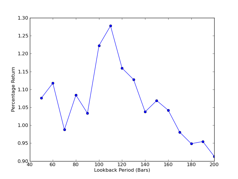
SPY-IWM linear regression hedge-ratio lookback period sensitivity analysis
No backtesting article would be complete without an upwardly sloping equity curve! Thus if you wish to plot a curve of the cumulated returns vs time, you can use the following code. It will plot the final portfolio generated from the lookback parameter study. Thus it will be necessary to choose the lookback depending upon which chart you wish to visualise. The chart also plots the returns of SPY in the same period to aid comparison:
            python

            # mr_spy_iwm.py

    # This is still within the main function
    print "Plotting the performance charts..."
    fig = plt.figure()
    fig.patch.set_facecolor('white')

    ax1 = fig.add_subplot(211,  ylabel='%s growth (%%)' % symbols[0])
    (pairs['%s_close' % symbols[0].lower()].pct_change()+1.0).cumprod().plot(ax=ax1, color='r', lw=2.)

    ax2 = fig.add_subplot(212, ylabel='Portfolio value growth (%%)')
    portfolio['returns'].plot(ax=ax2, lw=2.)

    fig.show()
The following equity curve chart is for a lookback period of 100 days:
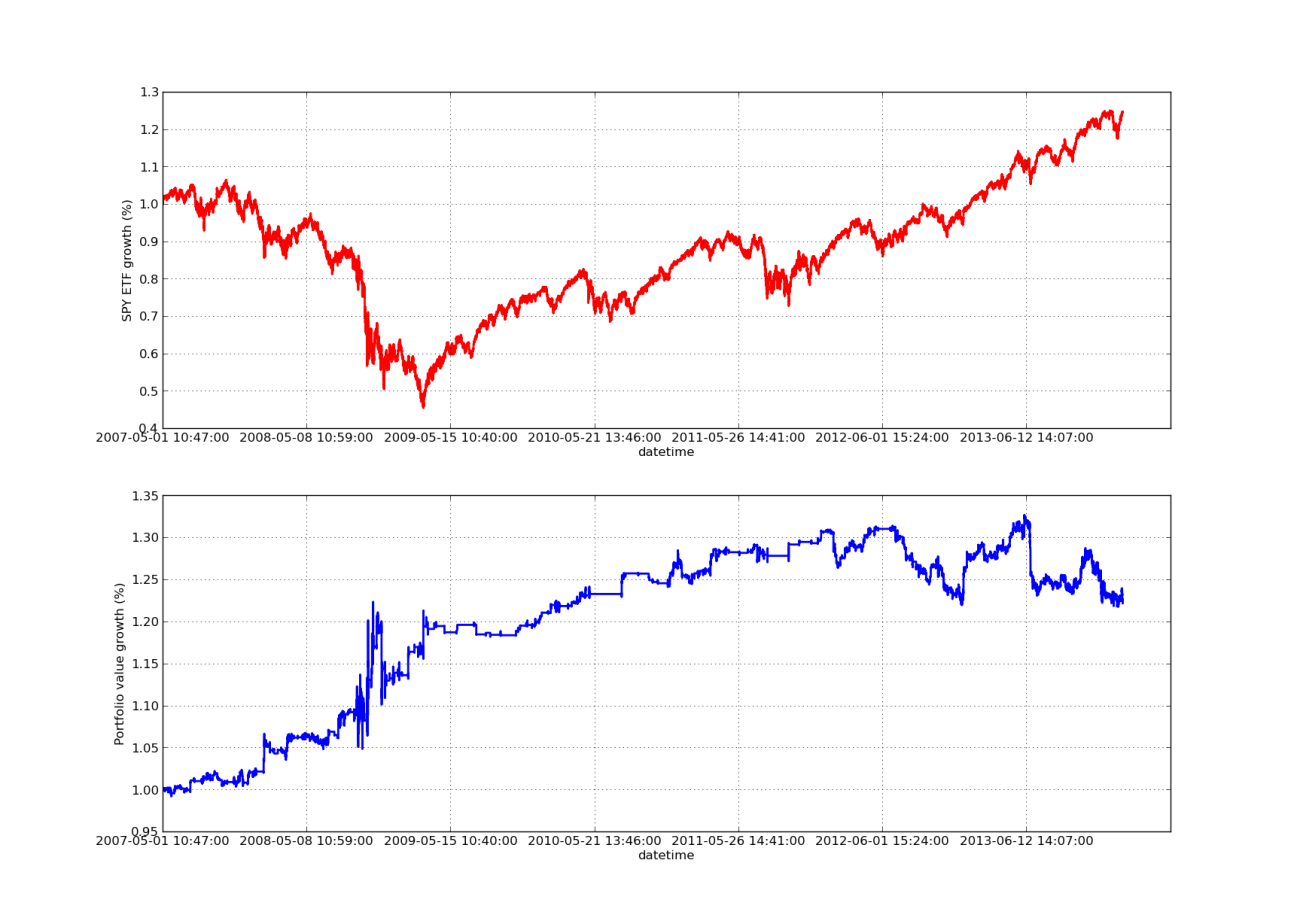
SPY-IWM linear regression hedge-ratio lookback period sensitivity analysis
Note that the drawdown of SPY is significant in 2009 during the period of the financial crisis. The strategy also had a volatile period at this stage. Also note that performance has deteriorated somewhat in the last year due to the strongly trending nature of SPY in this period, which reflects the S&P500 index.
Note that we still have to take into account the lookahead bias when calculating the z-score of the spread. Further, all of these calculations have been carried out without transaction costs. This strategy would certainly perform very poorly once these factors are taken into consideration. Fees, bid/ask spread and slippage are all currently unaccounted for. In addition the strategy is trading in fractional units of ETFs, which is also very unrealistic.
In later articles we will create a much more sophisticated event-driven backtester that will take these factors into consideration and give us significantly more confidence in our equity curve and performance metrics.
- 1