Advanced Platform Research — Python Data Analysis & Strategy Backtest

Advanced Platform Research — Python Data Analysis & Strategy Backtest.ipynb

Advanced Platform Research

FMZ has a built-in jupyter notebook to help users familiarize themselves with the platform API and conduct strategy research, and supports the learning environments of Python3 C++11/17 and Javascript. Notebook+Python is a very powerful tool, which is almost indispensable for data analysis and strategy research. Although the backtest that comes with the FMZ platform is very useful, it is not suitable for strategies with complex and large data volumes. This article will introduce some advanced using skills of jupyter notebook, and realize backtests of random trading pair and multi-trading pair strategies.

Use of Jupyter

The research environment inside FMZ can be used, but the networking is inconvenient. It is recommended to install on your own device the anaconda3, with notebook and commonly used related libraries for mathematical calculations; it can share the local network environment, and have better performance. It is also recommended to use Google colab. Although there are some storage limitations, it is free and powerful, suitable for the research related to robot studying .

Tutorial

There are many online tutorials for specific using skills of notebook and Python. You can find a lot of information by searching for keywords, like Python quantification and jupyter notebook tutorial. You need to learn and master a series of basics such as crawler, data processing, backtest, strategy design, and plotting.

Data Acquisition

Platforms generally provide APIs to obtain K-lines with history data, and some also provide data of execution trade by trade. We need to use the crawler to get and save the data. You can also directly receive the data pushed by the platform and create a local database storage by yourself.

Next, we will demonstrate how to obtain and store the K-line data of perpetual contracts on Binance.

First, find Binance Perpetual Swap documentation: https://binance-docs.github.io/apidocs/futures/cn/#c59e471e81 . You can see the required parameters and the returned data formats. Usually, the number of K-lines acquired by API is limited, and Binance has a maximum of 1000, so it needs to be acquired by loop iteration. The situation on other platforms is similar to Binance. Note that the network needs to be connected to the overseas network (compared to the domestic network in China) to crawl the K-lines.

The periods Binance supports:1m, 3m, 5m, 15m, 30m, 1h, 2h, 4h, 6h, 8h, 12h, 1d, 3d, 1w, 1M.

In [24]: import requests #network requests for the common library from datetime import date,datetime import time import pandas as pd In [160]: def GetKlines(symbol=‘BTC’,start=‘2020-8-10’,end=‘2021-8-10’,period=‘1h’): Klines = [] start_time = int(time.mktime(datetime.strptime(start, “%Y-%m-%d”).timetuple()))*1000 end_time = int(time.mktime(datetime.strptime(end, “%Y-%m-%d”).timetuple()))*1000 while start_time < end_time: res = requests.get(‘https://fapi.binance.com/fapi/v1/klines?symbol=%sUSDT&interval=%s&startTime=%s&limit=1000’%(symbol,period,start_time)) res_list = res.json() Klines += res_list #print(datetime.utcfromtimestamp(start_time/1000).strftime(’%Y-%m-%d %H:%M:%S’) ,len(res_list)) start_time = res_list[-1][0] return pd.DataFrame(Klines,columns=[‘time’,‘open’,‘high’,‘low’,‘close’,‘amount’,‘end_time’,‘volume’,‘count’,‘buy_amount’,‘buy_volume’,‘null’]).astype(‘float’) In [85]: df = GetKlines(symbol=‘BTC’,start=‘2021-1-1’,end=‘2021-8-10’,period=‘1h’)

Data storage and reading can use the functions inside pandas library. The format is csv, which can be directly opened with excel software.

In addition to the highest price, the lowest price, open price, close price and executed volume, the K-line data returned by Binance also includes the total trading amount, initiative buying amount, execution amount, etc. These is valuable information that can be used to construct strategies.

In [86]: df.to_csv(‘btc_klines.csv’) df = pd.read_csv(‘btc_klines.csv’,index_col=0) In [87]: df Out[87]: , , , , , , , , , , , , , , , , , , , , , , , , , , , , , , , , , , , , , , , , , , , , , , , , , , , , , , , , , , , , , , , , , , , , , , , , , , , , , , , , , , , , , , , , , , , , , , , , , , , , , , , , , , , , , , , , , , , , , , , , , , , , , , , , , , , , , , , , , , , , , , , , , , , , , , , , , , , , , , , , , , , , , , , , , , , , , , , , , , , , , , , , , , , time open high low close amount end_time volume count buy_amount buy_volume null 0 1596988800000 11575.08 11642.00 11566.07 11591.37 6541.466 1596992399999 7.592336e+07 25724 3127.898 3.630633e+07 0 1 1596992400000 11591.39 11610.23 11526.90 11534.39 6969.252 1596995999999 8.057780e+07 27403 3390.424 3.920162e+07 0 2 1596996000000 11534.39 11656.69 11527.93 11641.07 6439.365 1596999599999 7.469135e+07 25403 3446.186 3.997906e+07 0 3 1596999600000 11641.06 11665.90 11624.20 11635.30 3911.582 1597003199999 4.555459e+07 17820 1842.413 2.145768e+07 0 4 1597003200000 11635.29 11684.00 11635.29 11673.81 3461.004 1597006799999 4.036804e+07 15513 1660.575 1.936981e+07 0 … … … … … … … … … … … … … 8805 1628658000000 45627.72 45894.53 45540.00 45801.45 10296.202 1628661599999 4.710187e+08 112187 4988.565 2.282399e+08 0 8806 1628661600000 45801.46 46270.00 45800.01 46087.86 26409.962 1628665199999 1.215164e+09 247170 13696.301 6.302708e+08 0 8807 1628665200000 46087.87 46450.00 46087.87 46367.38 23969.309 1628668799999 1.110210e+09 232348 11990.951 5.554267e+08 0 8808 1628668800000 46367.37 46643.13 46002.01 46217.01 23472.769 1628672399999 1.086549e+09 229533 12334.292 5.711837e+08 0 8809 1628672400000 46217.01 46329.69 46046.54 46297.16 6579.477 1628675999999 3.039580e+08 78812 3313.055 1.530718e+08 0 , 8810 rows × 12 columns

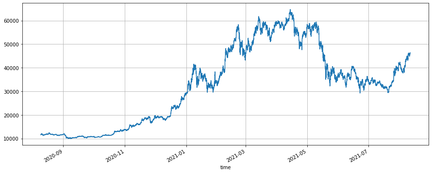
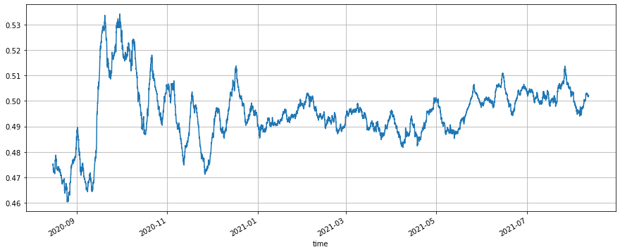
, In [88]: df.index = pd.to_datetime(df.time,unit=‘ms’) #convert the index into a date, which is convenient for plotting In [89]: df.close.plot(figsize=(15,6),grid = True); #close price Out[89]: In [92]: (df.buy_amount.rolling(150).mean()/df.amount.rolling(150).mean()).plot(figsize=(15,6),grid = True); #after flat, the proportion of initiative buy amount #the situation that the proportion of initiative buy amount rises after hitting the rock bottom normally responds to the situation of price increase, but the long-time average of the proportion of initiative buy amount is at 49% Out[92]: 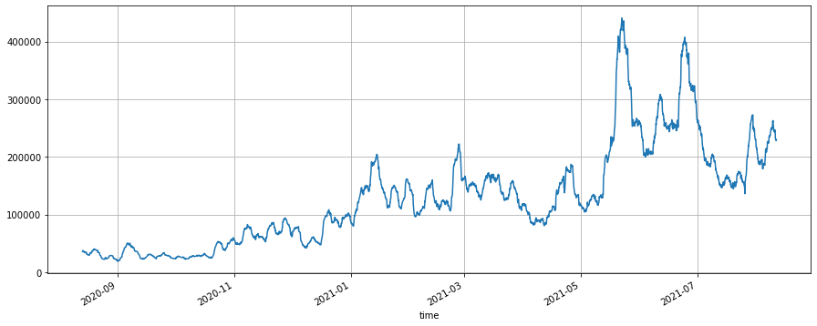In [93]: (df[‘count’].rolling(100).mean()).plot(figsize=(15,6),grid = True); #the executed amount after flat,and the market quotes might be prepared at a low location Out[93]:

Backtest Engine

The previous article also gave the Python backtest engine, but here is an optimized version. USDT-margined (or other quote currency-margined) perpetual contracts are very similar to spot contracts. The difference is that perpetual contracts can be leveraged and hold negative amount (equivalent to making short), and can share a backtest engine. crypto-margined delivery contracts are special, for they are settled in currency and require specific backtest.

Here a simple example is given, which can implement multi-symbol spot or multi-symbol perpetual backtesting. Many details are ignored: such as leverage of futures, margin occupation, funding rate, liquidation mechanism, market making and order taker transactions as well as order maintenance, but it usually does not affect the normal backtest results. And the price and quantity of the matching, and the account update all need to be imported externally. Readers can improve it on this basis.

Exchange class introduction:

• account:USDT indicates the base currency, which is not necessary; realised_profit: the profit and loss already realized; unrealised_profit: the profit and loss not realized yet; total: the total equity; fee: the handling fee. For other trading pairs, amount (which is negative number when making short); hold_price: the holding price; value: the holding value; price: the current price.

• trade_symbols: array of trading pairs; you can also pass in one trading pair; the default quote currency is USDT, but you can also use other quote currency symbols to backtest.

• fee: the handing fee; to be simple, do not distinguish maker and taker.

• initial_balance: the initial assets; the initial amount of the default trading pairs is 0.

• Buy function: to buy, which is corresponding to making long and closing short of perpetual contracts, without a matching mechanism.

• Sell function: to sell.

• Update function: to update the account information, which needs to pass in the price dictionary of all trading pairs. In [98]: class Exchange:

  def init(self, trade_symbols, fee=0.0004, initial_balance=10000): self.initial_balance = initial_balance #initial balance self.fee = fee self.trade_symbols = trade_symbols self.account = {‘USDT’:{‘realised_profit’:0, ‘unrealised_profit’:0, ‘total’:initial_balance, ‘fee’:0}} for symbol in trade_symbols: self.account[symbol] = {‘amount’:0, ‘hold_price’:0, ‘value’:0, ‘price’:0, ‘realised_profit’:0,‘unrealised_profit’:0,‘fee’:0}

  def Trade(self, symbol, direction, price, amount):

    cover_amount = 0 if direction*self.account[symbol]['amount'] >=0 else min(abs(self.account[symbol]['amount']), amount)
    open_amount = amount - cover_amount
    self.account['USDT']['realised_profit'] -= price*amount*self.fee #take out the fee 
    self.account['USDT']['fee'] += price*amount*self.fee
    self.account[symbol]['fee'] += price*amount*self.fee
  
    if cover_amount > 0: #close first 
        self.account['USDT']['realised_profit'] += -direction*(price - self.account[symbol]['hold_price'])*cover_amount  #profit 
        self.account[symbol]['realised_profit'] += -direction*(price - self.account[symbol]['hold_price'])*cover_amount
        
        self.account[symbol]['amount'] -= -direction*cover_amount
        self.account[symbol]['hold_price'] = 0 if self.account[symbol]['amount'] == 0 else self.account[symbol]['hold_price']
        
    if open_amount > 0:
        total_cost = self.account[symbol]['hold_price']*direction*self.account[symbol]['amount'] + price*open_amount
        total_amount = direction*self.account[symbol]['amount']+open_amount
        
        self.account[symbol]['hold_price'] = total_cost/total_amount
        self.account[symbol]['amount'] += direction*open_amount
  

  def Buy(self, symbol, price, amount): self.Trade(symbol, 1, price, amount)

  def Sell(self, symbol, price, amount): self.Trade(symbol, -1, price, amount)

  def Update(self, close_price): #update the assets self.account[‘USDT’][‘unrealised_profit’] = 0 for symbol in self.trade_symbols: self.account[symbol][‘unrealised_profit’] = (close_price[symbol] - self.account[symbol][‘hold_price’])*self.account[symbol][‘amount’] self.account[symbol][‘price’] = close_price[symbol] self.account[symbol][‘value’] = abs(self.account[symbol][‘amount’])*close_price[symbol] self.account[‘USDT’][‘unrealised_profit’] += self.account[symbol][‘unrealised_profit’] self.account[‘USDT’][‘total’] = round(self.account[‘USDT’][‘realised_profit’] + self.initial_balance + self.account[‘USDT’][‘unrealised_profit’],6) In [117]: #In the test, you can see that there is no emphasis on whether the platform is USDT-margined or spot. In fact, the result is the same, which is the reason for no distinction. e = Exchange([‘BTC’], fee=0.0004, initial_balance=10000) #create an Exchange object, and only one trading pair of BTC e.Buy(‘BTC’,40000, 0.1)#buy 0.1 BTC at the price of 40,000 e.Sell(‘BTC’,41000, 0.1)#sell 0.1 BTC at the price of 41,000 e.Update({‘BTC’:41000}) #updtae the account information print(e.account) #the final account information print('Profit: ',round(e.account[‘USDT’][‘total’]-e.initial_balance,2)) Out[117]:{‘USDT’: {‘realised_profit’: 96.76, ‘unrealised_profit’: 0.0, ‘total’: 10096.76, ‘fee’: 3.24}, ‘BTC’: {‘amount’: 0.0, ‘hold_price’: 0, ‘value’: 0.0, ‘price’: 41000, ‘realised_profit’: 100.0, ‘unrealised_profit’: 0.0, ‘fee’: 3.24}} profit： 96.76

Grid Strategy Backtest

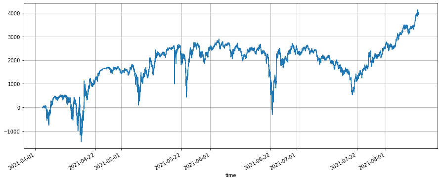
First, let’s backtest a classic perpetual grid strategy. This strategy is very popular on our platform recently. Compared with the spot grid one, it does not need to hold currency and can add leverage, which is much more convenient than the spot grid one. However, since it cannot be directly backtested, it is not conducive to select currency symbols. Here we use the backtest engine just now to test it.

On the top of “Live”, there is an official bot, started from April 4, 2021; the position value is 150, the grid spacing is 0.01, and the current profit is 3600USDT. Using the same parameters and the 5min K-line to backtest, the profit is 3937USDT. Since the position value at the beginning of the bot is less than 150 USDT, the result is quite accurate. If you change the grid spacing to 0.005, the gain will be 5226U. A grid spacing of 0.005 is obviously a better parameter than 0.01, which needs to be backtested to find out.

The shorter the K-line period, the more accurate the corresponding backtest results, and the larger the amount of data required. Readers can try changing the symbol parameter to the trading pair they want to backtest.

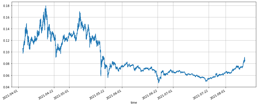
In [241]: symbol = ‘TRX’ df = GetKlines(symbol=symbol,start=‘2021-4-4’,end=‘2021-8-11’,period=‘5m’) In [286]: value = 150 pct = 0.01

e = Exchange([symbol], fee=0.0002, initial_balance=10000) init_price = df.loc[0,‘close’] res_list = [] #used to store the middle result for row in df.iterrows(): kline = row[1] #that will only test one K-line and only get one buy order or one sell order, which is not very accurate buy_price = (value / pct - value) / ((value / pct) / init_price + e.account[symbol][‘amount’]) #sell order price, for it is a maker execution, is also the final matching price sell_price = (value / pct + value) / ((value / pct) / init_price + e.account[symbol][‘amount’])

if kline.low < buy_price: #the lowest price of K-line is less than the current maker price; the buy order is executed 
    e.Buy(symbol,buy_price,value/buy_price)
if kline.high > sell_price:
    e.Sell(symbol,sell_price,value/sell_price)
e.Update({symbol:kline.close})
res_list.append([kline.time, kline.close, e.account[symbol]['amount'], e.account['USDT']['total']-e.initial_balance])

res = pd.DataFrame(data=res_list, columns=[‘time’,‘price’,‘amount’,‘profit’]) res.index = pd.to_datetime(res.time,unit=‘ms’) In [287]: e.account Out[287]:{‘USDT’: {‘realised_profit’: 3866.633149565143, ‘unrealised_profit’: 70.54622281993666, ‘total’: 13937.179372, ‘fee’: 177.51000000000596}, ‘TRX’: {‘amount’: 36497.43208747655, ‘hold_price’: 0.08203709078461048, ‘value’: 3064.689372385406, ‘price’: 0.08397, ‘realised_profit’: 4044.143149565462, ‘unrealised_profit’: 70.54622281993666, ‘fee’: 177.51000000000596}} In [288]: res.profit.plot(figsize=(15,6),grid = True); Out[288]: In [170]: res.price.plot(figsize=(15,6),grid = True); #close price Out[170]:

Spot Equilibrium Strategy Backtest

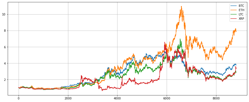
This type of strategy is also relatively popular, but FMZ platform is not very good at backtesting multi-symbol strategies, just use this backtest engine to have a try. We select four mainstream currency symbols, BTC, ETH, LTC, and XRP, and configure 25% of the market value respectively, and balance every 1% deviation.

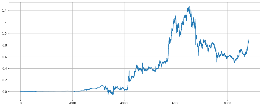
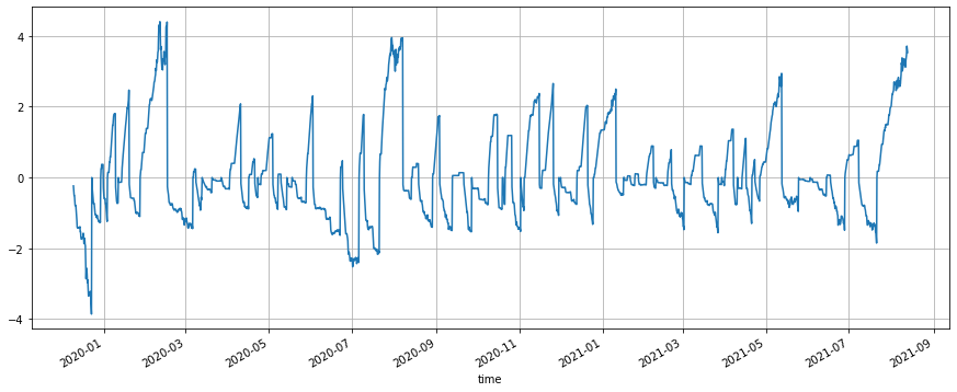
First, obtain the close prices of the four symbols in the past year. It can be seen that ETH has the largest increase, and the other three have similar increases. If you hold these four symbols on average, the final net value is 4.5. After backtest, the equilibrium strategy has a final net value of 5.3, which is slightly enhanced.

In [290]: symbols = [‘BTC’,‘ETH’,‘LTC’,‘XRP’] data = {} for symbol in symbols: df = GetKlines(symbol=symbol,start=‘2020-8-11’,end=‘2021-8-11’,period=‘1h’) data[symbol] = df.close In [291]: df = pd.DataFrame([data[symbol].values for symbol in symbols],index=symbols).T In [302]: e = Exchange(symbols, fee=0.0004, initial_balance=10000) res_list = [] for row in df.iterrows(): prices = row[1] total = e.account[‘USDT’][‘total’] e.Update(prices) for symbol in symbols: pct = e.account[symbol][‘value’]/total if pct > 0.26: e.Sell(symbol,prices[symbol],(pct-0.25)*total/prices[symbol]) if pct < 0.24: e.Buy(symbol,prices[symbol],(0.25-pct)*total/prices[symbol]) res_list.append([e.account[symbol][‘value’] for symbol in symbols] + [e.account[‘USDT’][‘total’]]) res = pd.DataFrame(data=res_list, columns=symbols+[‘total’]) In [303]: (df/df.iloc[0,:]).plot(figsize=(15,6),grid = True); #plot the trand by normalization Out[303]: In [304]: (res.total/10000-(df/df.iloc[0,:]).mean(axis=1)).plot(figsize=(15,6),grid = True); #enheance the effect Out[304]:

Turtle Strategy

The turtle strategy is a classic trend strategy, which includes complete stop-loss logic for adding positions. For details, please refer to: https://zhuanlan.zhihu.com/p/27987938 . We will implement a simple version here for backtest.

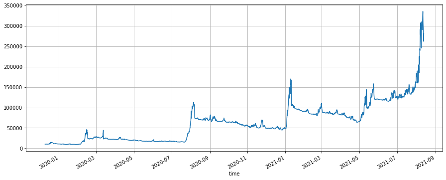
The turtle strategy period has a great influence on the strategy, and it is inadvisable to choose a period that is too short. Here, we choose 6h. The Donchian channel period is selected as 5, and the position ratio is selected as 0.003 according to the backtest. When the price breaks through the upBand of the channel to open 1 unit of long position, and the price continues to rise by 0.3 volatility after opening the positions, continue to add 1 unit, and the price falls below 2.5 Volatility of the latest open price to stop loss. The principle of short order is the same. Due to the large bull market of ETH, the turtle strategy has captured the main trend and eventually achieved 27 times of profits, with a maximum leverage of 4 times during the period.

The parameters of the turtle strategy are closely related to the period, and they need to be selected through backtest. The unit of each time’s open position should also be careful not to be too large to avoid over high risks.

It can be seen from the final net value chart that the turtle strategy is a long-term strategy, during which there may be no profit for 3 to 4 months, and repeated stopping loss, but once there is a big market quote on one side, the turtle strategy can take advantage of the trend to accumulate a large position, hold it to the end of the trend, earn a lot of profits. At the end of the rise, the strategy will accumulate a lot of positions. At this time, the volatility will be relatively large, and often large profits will be withdrawn. Using the turtle strategy requires you to accept its shortcomings and your patience.

In [424]: symbol = ‘ETH’ df = GetKlines(symbol=symbol,start=‘2019-8-11’,end=‘2021-8-11’,period=‘6h’) In [425]: df.index = pd.to_datetime(df.time,unit=‘ms’) In [568]: M = 5 # period volume of Donchian channel pct = 0.003 #the proportion of the added positions in the total positions df[‘up’] = df[‘high’].rolling(M).max().shift(1) #upBand of Donchian channel, used to make long and judge to break through t df[‘down’] = df[‘low’].rolling(M).max().shift(1) df[‘middle’] = (df[‘up’]+df[‘down’])/2 df[‘true_range’] = pd.concat([df[‘high’]-df[‘low’],df[‘high’]-df[‘close’].shift(1),df[‘close’].shift(1)-df[‘low’]],axis=1).max(axis=1) df[‘N’] = df[‘true_range’].rolling(50).mean() #N equals the recent volatility, used to judging to buy in and stop loss In [572]: open_times = 0.3 #judgement of opening a position stop_times = 2.5 #stop loss e = Exchange([symbol], fee=0.0004, initial_balance=10000) #set the taker to 0.0004 res_list = [] last_price = 0 #last open position price for row in df.iterrows(): kline = row[1] if kline.isnull().sum() > 0: #skip the section without data continue unit = e.account[‘USDT’][‘total’]*pct/kline.N #open position unit amount

if kline.high >  kline.up and e.account[symbol]['amount'] == 0: #first time to open long position 
    e.Buy(symbol,kline.up,unit) #notice the trading price here
    last_price = kline.up
if e.account[symbol]['amount'] > 0 and kline.high > last_price + open_times*kline.N: #long position, buy in 
    e.Buy(symbol,last_price + open_times*kline.N,unit)
    last_price = last_price + open_times*kline.N
if e.account[symbol]['amount'] > 0 and kline.low < last_price - stop_times*kline.N: #long position, stop loss
    e.Sell(symbol,last_price - stop_times*kline.N,e.account[symbol]['amount'])
    
if kline.low <  kline.down and e.account[symbol]['amount'] == 0: #open short
    e.Sell(symbol,kline.down,unit)
    last_price = kline.down
if e.account[symbol]['amount'] < 0 and kline.low < last_price - open_times*kline.N: #short position, buy in 
    e.Sell(symbol,last_price - open_times*kline.N,unit)
    last_price = last_price - open_times*kline.N
if e.account[symbol]['amount'] < 0 and kline.high > last_price + stop_times*kline.N: #short position, stop loss
    e.Buy(symbol,last_price + stop_times*kline.N,-e.account[symbol]['amount'])
    
e.Update({symbol:kline.close})
res_list.append([kline.time, kline.close, e.account[symbol]['amount']*kline.close, e.account['USDT']['total']])

res = pd.DataFrame(data=res_list, columns=[‘time’,‘price’,‘value’,‘total’]) res.index = pd.to_datetime(res.time,unit=‘ms’) print(‘Final market value:’,res[‘total’][-1]) Out[572]:Final market value: 280760.566996 In [573]: res.total.plot(figsize=(15,6),grid = True); Out[573]: In [571]: (res.value/res.total).plot(figsize=(15,6),grid = True); Out[571]:

Conclusion

If you are proficient in using the jupyter notebook research platform, you can easily perform operations, like data acquisition, data analysis, strategy backtest, chart display, etc., which is the inevitable way to quantitative trading. If you don’t have a clue about strategy writing right now, you might as well analyze the data first. For beginners, recommended resources:

Use Python to perform data analysis: https://wizardforcel.gitbooks.io/pyda-2e/content/

Python quantitative tutorial: https://wizardforcel.gitbooks.io/python-quant-uqer/content/

In [ ]: