

Pair trading based on data-driven technology
Pair trading is a good example of formulating trading strategies based on mathematical analysis. In this article, we will demonstrate how to use data to create and automate pair trading strategies.
Basic principles
Suppose you have a pair of investment targets X and Y that have some potential connections. For example, two companies produce the same products, such as Pepsi Cola and Coca Cola. You want the price ratio or basis spreads (also known as price difference) of the two to remain unchanged over time. However, due to the temporary changes in supply and demand, such as a large buying/selling order of an investment target, and the reaction to the important news of one of the companies, the price difference between the two pairs may be different from time to time. In this case, one investment object moves up while the other moves down relative to each other. If you want this disagreement to return to normal over time, you can find trading opportunities (or arbitrage opportunities). Such arbitrage opportunities can be found everywhere in the digital currency market or domestic commodity futures market, such as the relationship between BTC and safe haven assets; The relationship between soybean meal, soybean oil and soybean varieties in futures.
When there is a temporary price difference, you will sell the investment object with excellent performance (the rising investment object) and buy the investment object with poor performance (the falling investment object). You are sure that the interest margin between the two investment objects will eventually fall through the fall of the investment object with excellent performance or the rise of the investment object with poor performance, or both. Your transaction will make money in all these similar situations. If the investment objects move up or down together without changing the price difference between them, you will not make or lose money.
Therefore, pair trading is a market neutral trading strategy, enabling traders to profit from almost any market conditions: upward trend, downward trend or horizontal consolidation.
Explain the concept: two hypothetical investment targets
- Build our research environment on the FMZ Quant platform
First of all, in order to work smoothly, we need to build our research environment. In this article, we use the FMZ Quant platform (FMZ.COM) to build our research environment, mainly to use the convenient and fast API interface and the well-packaged Docker system of this platform later.
In the official name of the FMZ Quant platform, this Docker system is called the Docker system.
Please refer to my previous article on how to deploy a docker and robot: https://www.fmz.com/bbs-topic/9864.
Readers who want to purchase their own cloud computing server to deploy dockers can refer to this article: https://www.fmz.com/digest-topic/5711.
After deploying the cloud computing server and the docker system successfully, next, we will install the present largest artifact of Python: Anaconda
In order to realize all the relevant program environments (dependency libraries, version management, etc.) required in this article, the simplest way is to use Anaconda. It is a packaged Python data science ecosystem and dependency library manager.
For the installation method of Anaconda, please refer to the official guide of Anaconda: https://www.anaconda.com/distribution/.
This article will also use numpy and pandas, two popular and important libraries in Python scientific computing.
The above basic work can also refer to my previous articles, which introduce how to set up the Anaconda environment and the numpy and pandas libraries. For details, please refer to: https://www.fmz.com/bbs-topic/9863.
Next, let's use code to implement a "two hypothetical investment target":
import numpy as np
import pandas as pd
import statsmodels
from statsmodels.tsa.stattools import coint
# just set the seed for the random number generator
np.random.seed(107)
import matplotlib.pyplot as plt
Yes, we will also use matplotlib, a very famous chart library in Python.
Let's generate a hypothetical investment target X, and simulate and plot its daily return through normal distribution. Then we perform a cumulative sum to get the daily X value.
            # Generate daily returns
Xreturns = np.random.normal(0, 1, 100)
# sum them and shift all the prices up
X = pd.Series(np.cumsum(
    Xreturns), name='X')
    + 50
X.plot(figsize=(15,7))
plt.show()
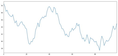
The X of the investment object is simulated to plot its daily return through a normal distribution
Now we generate Y, which is strongly integrated with X, so the price of Y should be very similar to the change of X. We model this by taking X, moving it up and adding some random noise extracted from the normal distribution.
            noise = np.random.normal(0, 1, 100)
Y = X + 5 + noise
Y.name = 'Y'
pd.concat([X, Y], axis=1).plot(figsize=(15,7))
plt.show()
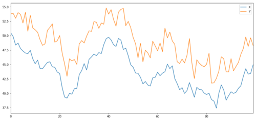
X and Y of cointegration investment object
Cointegration
Cointegration is very similar to correlation, which means that the ratio between two data series will change near the average value. The Y and X series follow the following:
Y = ⍺ X + e
Where ⍺ is a constant ratio and e is the noise.
For pairs trading between two time series, the expected value of the ratio over time must converge to the mean value, that is, they should be cointegrated. The time series we built above is cointegrated. We will plot the ratio between them now so that we can see what it looks like.
            (Y/X).plot(figsize=(15,7))
plt.axhline((Y/X).mean(), color='red', linestyle='--')
plt.xlabel('Time')
plt.legend(['Price Ratio', 'Mean'])
plt.show()
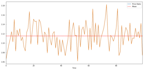
Ratio and average value between two co-integrated investment target prices
Cointegration test
A convenient test method is to use statsmodels.tsa.stattools. We will see a very low p value, because we created two data series artificially that are as co-integrated as possible.
            # compute the p-value of the cointegration test
# will inform us as to whether the ratio between the 2 timeseries is stationary
# around its mean
score, pvalue, _ = coint(X,Y)
print pvalue
The result is: 1.81864477307e-17
Note: correlation and cointegration
Correlation and cointegration, although similar in theory, are not the same. Let's look at examples of relevant but not co-integrated data series and vice versa. First, let's check the correlation of the series we just generated.
X.corr(Y)
The result is : 0.951
As we expected, this is very high. But what about two related but not co-integrated series? A simple example is a series of two deviating data.
            ret1 = np.random.normal(1, 1, 100)
ret2 = np.random.normal(2, 1, 100)

s1 = pd.Series( np.cumsum(ret1), name='X')
s2 = pd.Series( np.cumsum(ret2), name='Y')

pd.concat([s1, s2], axis=1 ).plot(figsize=(15,7))
plt.show()
print 'Correlation: ' + str(X_diverging.corr(Y_diverging))
score, pvalue, _ = coint(X_diverging,Y_diverging)
print 'Cointegration test p-value: ' + str(pvalue)
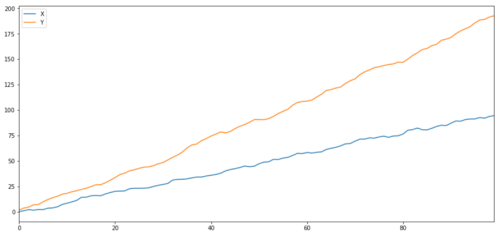
Two related series (not integrated together)
Correlation coefficient: 0.998
P value of cointegration test: 0.258
Simple examples of cointegration without correlation are normal distribution sequences and square waves.
            Y2 = pd.Series(np.random.normal(0, 1, 800), name='Y2') + 20
Y3 = Y2.copy()
Y3[0:100] = 30
            Y3[100:200] = 10
Y3[200:300] = 30
Y3[300:400] = 10
Y3[400:500] = 30
Y3[500:600] = 10
Y3[600:700] = 30
Y3[700:800] = 10
Y2.plot(figsize=(15,7))
Y3.plot()
plt.ylim([0, 40])
plt.show()
# correlation is nearly zero
print 'Correlation: ' + str(Y2.corr(Y3))
score, pvalue, _ = coint(Y2,Y3)
print 'Cointegration test p-value: ' + str(pvalue)
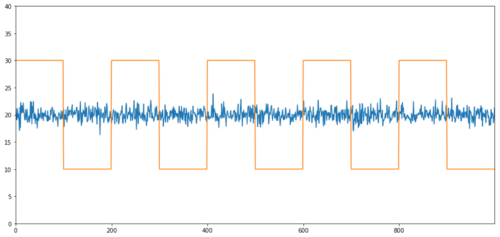
Correlation: 0.007546
P value of cointegration test: 0.0
The correlation is very low, but the p value shows perfect co-integration!
How to conduct pair trading?
Because two co-integrated time series (such as X and Y above) are facing each other and deviating from each other, sometimes the basis spreads is high or low. We conduct pair trading by buying one investment object and selling another. In this way, if the two investment targets fall or rise together, we will neither make money nor lose money, that is, we are neutral in the market.
Back to the above, X and Y in Y = ⍺ X + e, so that the ratio (Y/X) moves around its average value ⍺. We make money through the ratio of average value reversion. To do this, we will pay attention to the case where X and Y are far apart, that is, the value of ⍺ is too high or too low:
-
Going long ratio: This is when the ratio ⍺ is very small and we expect it to increase. In the above example, we open the position by going long Y and going short X.
-
Going short ratio: This is when the ratio ⍺ is very large and we expect it to decrease. In the above example, we open the position by going short Y and going long X.
Please note that we always have a "hedge position": if the trading subject buys loss value, the short position will make money, and vice versa, so we are immune to the overall market trend.
If the X and Y of the trading object move relative to each other, we will make money or lose money.
Use data to find trading objects with similar behavior
The best way to do this is to start from the trading subject that you suspect may be co-integration and perform a statistical test. If you conduct statistical tests on all trading pairs, you will become a victim of multiple comparison bias.
Multiple comparison bias refers to the increased chance of incorrectly generating important p values when running many tests, because we need to run a large number of tests. If we run 100 tests on random data, we should see 5 p values below 0.05. If you want to compare n trading targets for co-integration, you will perform n (n-1)/2 comparisons, and you will see many incorrect p values, which will increase with the increase of your test samples. To avoid this situation, select a few trading pairs and you have reason to determine that they may be co-integration, and then test them separately. This will greatly reduce multiple comparison bias.
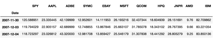
Therefore, let's try to find some trading targets that show co-integration. Let's take a basket of large US technology stocks in the S&P 500 Index as an example. These trading targets operate in similar market segments and have co-integration prices. We scan the list of trading objects and test the co-integration between all pairs.
The returned co-integration test score matrix, p-value matrix and all pairs with p-value less than 0.05. This method is prone to multiple comparison bias, so in fact, they need to conduct a second verification. In this article, for the convenience of our explanation, we choose to ignore this point in the example.
            def find_cointegrated_pairs(data):
    n = data.shape[1]
    score_matrix = np.zeros((n, n))
    pvalue_matrix = np.ones((n, n))
    keys = data.keys()
    pairs = []
    for i in range(n):
        for j in range(i+1, n):
            S1 = data[keys[i]]
            S2 = data[keys[j]]
            result = coint(S1, S2)
            score = result[0]
            pvalue = result[1]
            score_matrix[i, j] = score
            pvalue_matrix[i, j] = pvalue
            if pvalue < 0.02:
                pairs.append((keys[i], keys[j]))
    return score_matrix, pvalue_matrix, pairs
Note: We have included the market benchmark (SPX) in the data - the market has driven the flow of many trading objects. Usually you may find two trading objects that appear to be cointegrated; But in fact, they do not co integrate with each other, but with the market. This is called a confounding variable. It is important to check market participation in any relationship you find.
            from backtester.dataSource.yahoo_data_source import YahooStockDataSource
from datetime import datetime
startDateStr = '2007/12/01'
endDateStr = '2017/12/01'
cachedFolderName = 'yahooData/'
dataSetId = 'testPairsTrading'
instrumentIds = ['SPY','AAPL','ADBE','SYMC','EBAY','MSFT','QCOM',
                 'HPQ','JNPR','AMD','IBM']
ds = YahooStockDataSource(cachedFolderName=cachedFolderName,
                            dataSetId=dataSetId,
                            instrumentIds=instrumentIds,
                            startDateStr=startDateStr,
                            endDateStr=endDateStr,
                            event='history')
data = ds.getBookDataByFeature()['Adj Close']
data.head(3)
Now let's try to use our method to find cointegrated trading pairs.
            # Heatmap to show the p-values of the cointegration test
# between each pair of stocks
scores, pvalues, pairs = find_cointegrated_pairs(data)
import seaborn
m = [0,0.2,0.4,0.6,0.8,1]
seaborn.heatmap(pvalues, xticklabels=instrumentIds,
                yticklabels=instrumentIds, cmap=’RdYlGn_r’,
                mask = (pvalues >= 0.98))
plt.show()
print pairs
[('ADBE', 'MSFT')]

It looks like 'ADBE' and 'MSFT' are cointegrated. Let's take a look at the price to make sure it really makes sense.
            S1 = data['ADBE']
S2 = data['MSFT']
score, pvalue, _ = coint(S1, S2)
print(pvalue)
ratios = S1 / S2
ratios.plot()
plt.axhline(ratios.mean())
plt.legend([' Ratio'])
plt.show()
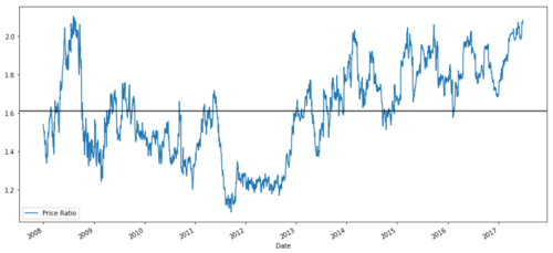
Price ratio chart between MSFT and ADBE from 2008 to 2017
This ratio does look like a stable average. Absolute ratios are not statistically useful. It is more helpful to standardize our signals by treating them as Z Score. The Z Score is defined as:
Z Score (Value) = (Value — Mean) / Standard Deviation
Warning
In fact, we usually try to expand the data on the premise that the data is normally distributed. However, many financial data are not normally distributed, so we must be very careful not to simply assume normality or any specific distribution when generating statistics. The true distribution of ratios may have a fat-tail effect, and those data that tend to be extreme will confuse our model and lead to huge losses.
            def zscore(series):
    return (series - series.mean()) / np.std(series)
            zscore(ratios).plot()
plt.axhline(zscore(ratios).mean())
plt.axhline(1.0, color=’red’)
plt.axhline(-1.0, color=’green’)
plt.show()
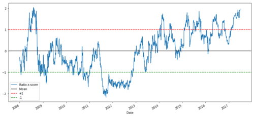
Z price ratio between MSFT and ADBE from 2008 to 2017
Now it is easier to observe the movement of the ratio near the average value, but sometimes it is easy to have a big difference from the average value. We can take advantage of this.
Now that we have discussed the basic knowledge of pair trading strategy, and determined the subject matter of joint integration based on the historical price, let's try to develop a trading signal. First, let's review the steps of developing trading signals by using data technology:
-
Collect reliable data and clean up data;
-
Create functions from data to identify trading signals/logic;
-
Functions can be moving averages or price data, correlations or ratios of more complex signals - combine these to create new functions;
-
Use these functions to generate trading signals, that is, which signals are buying, selling or short position to watch.
Fortunately, we have the FMZ Quant platform (fmz.com), which has completed the above four aspects for us, which is a great blessing for strategy developers. We can devote our energy and time to the design of strategy logic and the extension of functions.
In the FMZ Quant platform, there are encapsulated interfaces for various mainstream exchanges. What we need to do is call these API interfaces. The rest of the underlying implementation logic has been finished by a professional team.
In order to complete the logic and explain the principle in this article, we will present these underlying logic in detail. However, in actual operation, readers can call the FMZ Quant API interface directly to complete the above four aspects.
Let's start:
Step 1: Set your question
Here, we try to create a signal to tell us whether the ratio will buy or sell at the next moment, that is, our prediction variable Y:
Y = Ratio is buy (1) or sell (-1)
Y(t)= Sign(Ratio(t+1) — Ratio(t))
Please note that we do not need to predict the actual transaction target price, or even the actual value of the ratio (although we can), but only the ratio direction in the next step.
Step 2: Collect reliable and accurate data
FMZ Quant is your friend! You only need to specify the transaction object to be traded and the data source to be used, and it will extract the required data and clear it for dividend and transaction object splitting. So the data here is very clean.
On the trading days of the past 10 years (about 2500 data points), we obtained the following data by using Yahoo Finance: opening price, closing price, highest price, lowest price and trading volume.
Step 3: Split the data
Don't forget this very important step in testing the accuracy of the model. We are using the following data for training/validation/test split.
-
Training 7 years ~ 70%
-
Test ~ 3 years 30%
            ratios = data['ADBE'] / data['MSFT']
print(len(ratios))
train = ratios[:1762]
test = ratios[1762:]
Ideally, we should also make validation sets, but we won't do that for now.
Step 4: Feature engineering
What can the related functions be? We want to predict the direction of the ratio change. We have seen that our two trading targets are cointegrated, so this ratio tends to shift and return to the average value. It seems that our characteristics should be some measures of the average ratio, and the difference between the current value and the average value can generate our trading signal.
We use the following functions:
-
60-day moving average ratio: measurement of rolling average;
-
5-day moving average ratio: measurement of the current value of the average;
-
60-day standard deviation;
-
Z Score: (5d MA - 60d MA) / 60d SD.
            ratios_mavg5 = train.rolling(window=5,
                               center=False).mean()
ratios_mavg60 = train.rolling(window=60,
                               center=False).mean()
std_60 = train.rolling(window=60,
                        center=False).std()
zscore_60_5 = (ratios_mavg5 - ratios_mavg60)/std_60
plt.figure(figsize=(15,7))
plt.plot(train.index, train.values)
plt.plot(ratios_mavg5.index, ratios_mavg5.values)
plt.plot(ratios_mavg60.index, ratios_mavg60.values)
plt.legend(['Ratio','5d Ratio MA', '60d Ratio MA'])
plt.ylabel('Ratio')
plt.show()
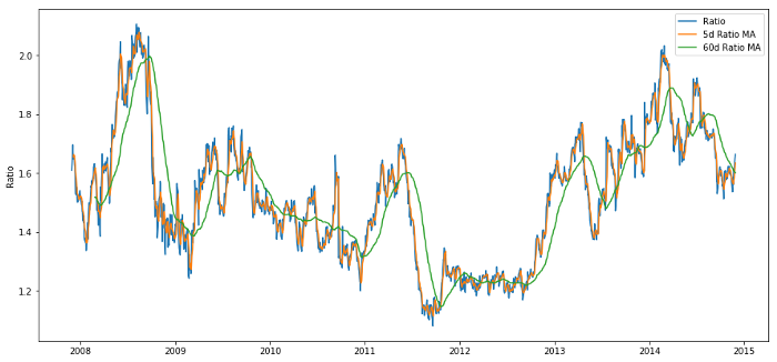
Price ratio between 60d and 5d MA
            plt.figure(figsize=(15,7))
zscore_60_5.plot()
plt.axhline(0, color='black')
plt.axhline(1.0, color='red', linestyle='--')
plt.axhline(-1.0, color='green', linestyle='--')
plt.legend(['Rolling Ratio z-Score', 'Mean', '+1', '-1'])
plt.show()
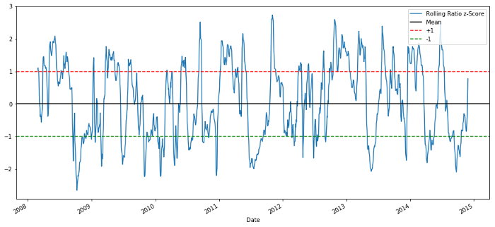
60-5 Z Score price ratios
The Z Score of the rolling average value does bring out the average value regression property of the ratio!
Step 5: Model selection
Let's start with a very simple model. Looking at the z score chart, we can see that if the z score is too high or too low, it will return. Let's use+1/- 1 as our threshold to define too high and too low, and then we can use the following model to generate trading signals:
-
When z is below - 1.0, the ratio is to buy (1), because we expect z to return to 0, so the ratio increases;
-
When z is above 1.0, the ratio is sell (- 1), because we expect z to return to 0, so the ratio decreases.
Step 6: Training, verification and optimization
Finally, let's take a look at the actual impact of our model on the actual data? Let's take a look at the performance of this signal on the actual ratio:
            # Plot the ratios and buy and sell signals from z score
plt.figure(figsize=(15,7))
train[60:].plot()
buy = train.copy()
sell = train.copy()
buy[zscore_60_5>-1] = 0
sell[zscore_60_5<1] = 0
buy[60:].plot(color=’g’, linestyle=’None’, marker=’^’)
sell[60:].plot(color=’r’, linestyle=’None’, marker=’^’)
x1,x2,y1,y2 = plt.axis()
plt.axis((x1,x2,ratios.min(),ratios.max()))
plt.legend([‘Ratio’, ‘Buy Signal’, ‘Sell Signal’])
plt.show()
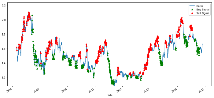
Buying and selling price ratio signal
The signal seems reasonable. We seem to sell when it is high or increasing (red dots) and buy it back when it is low (green dots) and decreasing. What does this mean for the actual subject matter of our transaction? Let's see:
            # Plot the prices and buy and sell signals from z score
plt.figure(figsize=(18,9))
S1 = data['ADBE'].iloc[:1762]
S2 = data['MSFT'].iloc[:1762]
S1[60:].plot(color='b')
S2[60:].plot(color='c')
buyR = 0*S1.copy()
sellR = 0*S1.copy()
# When buying the ratio, buy S1 and sell S2
buyR[buy!=0] = S1[buy!=0]
sellR[buy!=0] = S2[buy!=0]
# When selling the ratio, sell S1 and buy S2
buyR[sell!=0] = S2[sell!=0]
sellR[sell!=0] = S1[sell!=0]
buyR[60:].plot(color='g', linestyle='None', marker='^')
sellR[60:].plot(color='r', linestyle='None', marker='^')
x1,x2,y1,y2 = plt.axis()
plt.axis((x1,x2,min(S1.min(),S2.min()),max(S1.max(),S2.max())))
plt.legend(['ADBE','MSFT', 'Buy Signal', 'Sell Signal'])
plt.show()
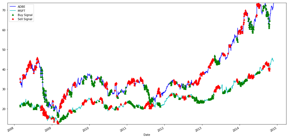
Signals to buy and sell MSFT and ADBE shares
Please pay attention to how we sometimes make profits on "short legs", sometimes on "long legs", and sometimes both.
We are satisfied with the signal of the training data. Let's see what kind of profit this signal can generate. When the ratio is low, we can make a simple back tester, buy a ratio (buy 1 ADBE stock and sell ratio x MSFT stock), and sell a ratio (sell 1 ADBE stock and buy x ratio MSFT stock) when it is high, and calculate the PnL transactions of these ratios.
            # Trade using a simple strategy
def trade(S1, S2, window1, window2):

    # If window length is 0, algorithm doesn't make sense, so exit
    if (window1 == 0) or (window2 == 0):
        return 0

    # Compute rolling mean and rolling standard deviation
    ratios = S1/S2
    ma1 = ratios.rolling(window=window1,
                               center=False).mean()
    ma2 = ratios.rolling(window=window2,
                               center=False).mean()
    std = ratios.rolling(window=window2,
                        center=False).std()
    zscore = (ma1 - ma2)/std

    # Simulate trading
    # Start with no money and no positions
    money = 0
    countS1 = 0
    countS2 = 0
    for i in range(len(ratios)):
        # Sell short if the z-score is > 1
        if zscore[i] > 1:
            money += S1[i] - S2[i] * ratios[i]
            countS1 -= 1
            countS2 += ratios[i]
            print('Selling Ratio %s %s %s %s'%(money, ratios[i], countS1,countS2))
        # Buy long if the z-score is < 1
        elif zscore[i] < -1:
            money -= S1[i] - S2[i] * ratios[i]
            countS1 += 1
            countS2 -= ratios[i]
            print('Buying Ratio %s %s %s %s'%(money,ratios[i], countS1,countS2))
        # Clear positions if the z-score between -.5 and .5
        elif abs(zscore[i]) < 0.75:
            money += S1[i] * countS1 + S2[i] * countS2
            countS1 = 0
            countS2 = 0
            print('Exit pos %s %s %s %s'%(money,ratios[i], countS1,countS2))


    return money
trade(data['ADBE'].iloc[:1763], data['MSFT'].iloc[:1763], 60, 5)
The result is: 1783.375
So this strategy seems to be profitable! Now, we can further optimize by changing the moving average time window, by changing the thresholds of buying/selling and close positions, and check the performance improvement of validation data.
We can also try more complex models, such as Logistic regression and SVM, to predict 1/- 1.
Now, let's advance this model, which brings us to:
Step 7: Backtest the test data
Here again, the FMZ Quant platform adopts a high-performance QPS/TPS backtesting engine to reproduce the historical environment truly, eliminate common quantitative backtesting pitfalls, and discover the deficiencies of strategies in time, so as to better help the real bot investment.
In order to explain the principle, this article still chooses to show the underlying logic. In practical application, we recommend readers to use the FMZ Quant platform. In addition to saving time, it is important to improve the fault tolerance rate.
The backtesting is simple. We can use the above function to view the PnL of test data.
trade(data['ADBE'].iloc[1762:], data['MSFT'].iloc[1762:], 60, 5)
The result is: 5262.868
The model did a great job! It became our first simple paired pair trading model.
Avoid overfitting
Before concluding the discussion, I would like to discuss overfitting in particular. Overfitting is the most dangerous trap in trading strategies. The over fitting algorithm may perform very well in the backtest but fail on the new invisible data - which means that it does not really reveal any trend of the data and has no real prediction ability. Let's give a simple example.
In our model, we use rolling parameters to estimate and optimize the time window length. We may decide to simply iterate over all possibilities, a reasonable length of time window, and choose the length of time according to the best performance of our model. Let's write a simple loop to score the length of the time window according to the pnl of the training data and find the best loop.
            # Find the window length 0-254
# that gives the highest returns using this strategy
length_scores = [trade(data['ADBE'].iloc[:1762],
                data['MSFT'].iloc[:1762], l, 5)
                for l in range(255)]
best_length = np.argmax(length_scores)
print ('Best window length:', best_length)
('Best window length:', 40)
Now we examine the performance of the model on the test data, and we find that this time window length is far from optimal! This is because our original choice clearly over-fitted the sample data.
            # Find the returns for test data
# using what we think is the best window length
length_scores2 = [trade(data['ADBE'].iloc[1762:],
                  data['MSFT'].iloc[1762:],l,5)
                  for l in range(255)]
print (best_length, 'day window:', length_scores2[best_length])
# Find the best window length based on this dataset,
# and the returns using this window length
best_length2 = np.argmax(length_scores2)
print (best_length2, 'day window:', length_scores2[best_length2])
            (40, 'day window:', 1252233.1395)
(15, 'day window:', 1449116.4522)
It is obvious that the sample data suitable for us will not always produce good results in the future. Just for testing, let's plot the length scores calculated from the two data sets:
            plt.figure(figsize=(15,7))
plt.plot(length_scores)
plt.plot(length_scores2)
plt.xlabel('Window length')
plt.ylabel('Score')
plt.legend(['Training', 'Test'])
plt.show()
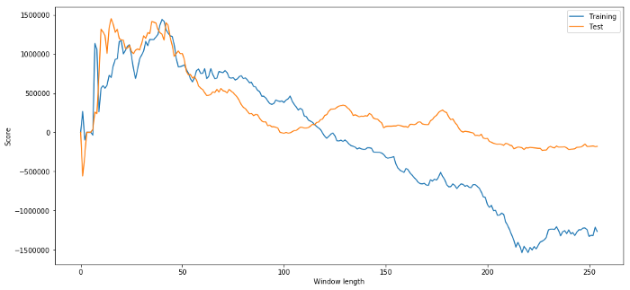
We can see that anything between 20 and 50 is a good choice item for time windows.
To avoid overfitting, we can use economic reasoning or the nature of the algorithm to select the length of the time window. We can also use Kalman filter, which does not require us to specify the length; This approach will be described later in another article.
Next step
In this article, we propose some simple introduction methods to demonstrate the process of developing trading strategies. In practice, more complex statistics should be used. You can consider the following options:
-
Hurst exponent;
-
Half life of mean regression inferred from Ornstein-Uhlenbeck process;
-
Kalman filter.
- 1