Thoughts on High-Frequency Trading Strategies (3)

In the previous article, I introduced how to model cumulative trading volume and analyzed the phenomenon of price impact. In this article, I will continue to analyze the trades order data. YGG recently launched Binance U-based contracts, and the price fluctuations have been significant, with trading volume even surpassing BTC at one point. Today, I will analyze it.

Order Time Intervals

In general, it is assumed that the arrival time of orders follows a Poisson process. There is an article that introduces the Poisson process . Here, I will provide empirical evidence.

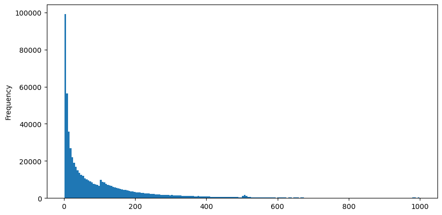
I downloaded the aggTrades data for August 5th, which consists of 1,931,193 trades, which is quite significant. First, let’s take a look at the distribution of buy orders. We can see a non-smooth local peak around 100ms and 500ms, which is likely caused by iceberg orders placed by trading bots at regular intervals. This may also be one of the reasons for the unusual market conditions that day.

The probability mass function (PMF) of the Poisson distribution is given by the following formula:

Where:

• κ is the number of events we are interested in.
• λ is the average rate of events occurring per unit time (or unit space).
• represents the probability of exactly κ events occurring, given the average rate λ.

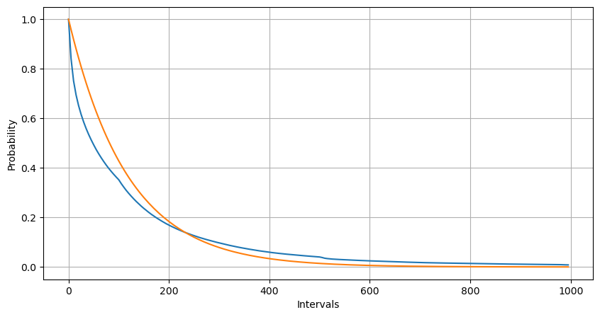
In a Poisson process, the time intervals between events follow an exponential distribution. The probability density function (PDF) of the exponential distribution is given by the following formula:

The fitting results show that there is a significant difference between the observed data and the expected Poisson distribution. The Poisson process underestimates the frequency of long time intervals and overestimates the frequency of short time intervals. (The actual distribution of intervals is closer to a modified Pareto distribution)

In [1]:

from datetime import date,datetime
import time
import pandas as pd
import numpy as np
import matplotlib.pyplot as plt
%matplotlib inline

In [2]:

trades = pd.read_csv('YGGUSDT-aggTrades-2023-08-05.csv')
trades['date'] = pd.to_datetime(trades['transact_time'], unit='ms')
trades.index = trades['date']
buy_trades = trades[trades['is_buyer_maker']==False].copy()
buy_trades = buy_trades.groupby('transact_time').agg({
    'agg_trade_id': 'last',
    'price': 'last',
    'quantity': 'sum',
    'first_trade_id': 'first',
    'last_trade_id': 'last',
    'is_buyer_maker': 'last',
    'date': 'last',
    'transact_time':'last'
})
buy_trades['interval']=buy_trades['transact_time'] - buy_trades['transact_time'].shift()
buy_trades.index = buy_trades['date']

In [10]:

buy_trades['interval'][buy_trades['interval']<1000].plot.hist(bins=200,figsize=(10, 5));

Out[10]:

In [20]:

Intervals = np.array(range(0, 1000, 5))
mean_intervals = buy_trades['interval'].mean()
buy_rates = 1000/mean_intervals
probabilities = np.array([np.mean(buy_trades['interval'] > interval)  for interval in Intervals])
probabilities_s = np.array([np.e**(-buy_rates*interval/1000) for interval in Intervals])

plt.figure(figsize=(10, 5))
plt.plot(Intervals, probabilities)
plt.plot(Intervals, probabilities_s)
plt.xlabel('Intervals')
plt.ylabel('Probability')
plt.grid(True)

Out[20]:

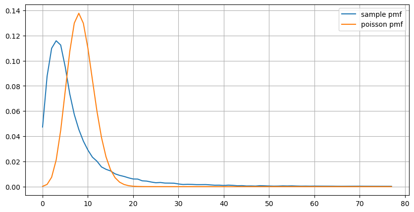
When comparing the distribution of the number of order occurrences within 1 second with the Poisson distribution, the difference is also significant. The Poisson distribution significantly underestimates the frequency of rare events. Possible reasons for this are:

• Non-constant rate of occurrence: The Poisson process assumes that the average rate of events occurring within any given time interval is constant. If this assumption does not hold, then the distribution of the data will deviate from the Poisson distribution.
• Interactions between processes: Another fundamental assumption of the Poisson process is that events are independent of each other. If events in the real world interact with each other, their distribution may deviate from the Poisson distribution.

In other words, in a real-world environment, the frequency of order occurrences is non-constant, and it needs to be updated in real-time. There may also be an incentive effect, where more orders within a fixed time period stimulate more orders. This makes strategies unable to rely on a single fixed parameter.

In [190]:

result_df = buy_trades.resample('1S').agg({ 
    'price': 'count',
    'quantity': 'sum'
}).rename(columns={'price': 'order_count', 'quantity': 'quantity_sum'})

In [219]:

count_df = result_df['order_count'].value_counts().sort_index()[result_df['order_count'].value_counts()>20]
(count_df/count_df.sum()).plot(figsize=(10,5),grid=True,label='sample pmf');

from scipy.stats import poisson
prob_values = poisson.pmf(count_df.index, 1000/mean_intervals) 

plt.plot(count_df.index, prob_values,label='poisson pmf');
plt.legend() ;

Out[219]:

Real-time Parameter Updating

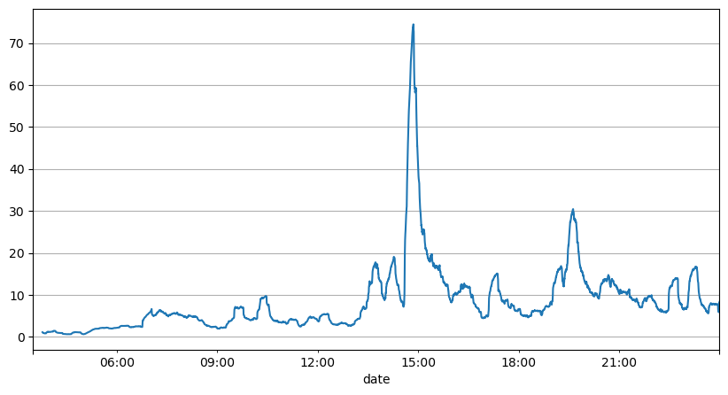
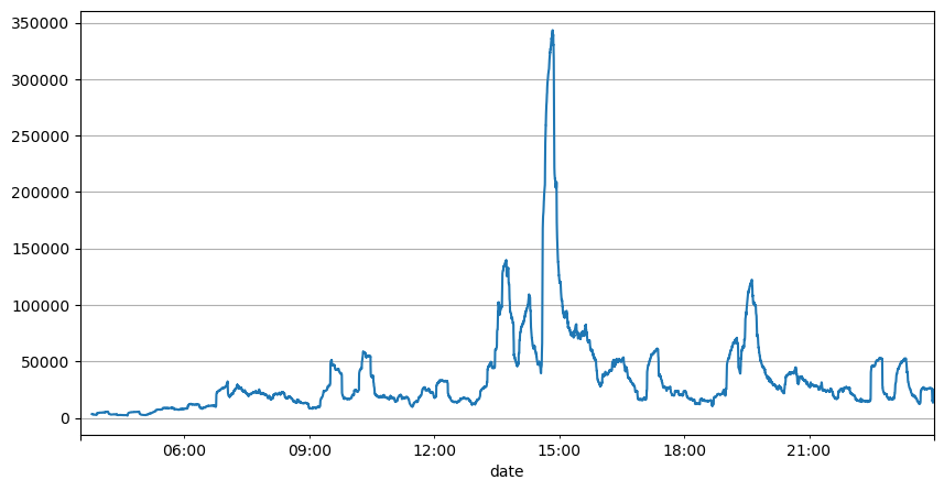
From the analysis of order intervals earlier, it can be concluded that fixed parameters are not suitable for the real market conditions, and the key parameters describing the market in the strategy need to be updated in real-time. The most straightforward solution is to use a sliding window moving average. The two graphs below show the frequency of buy orders within 1 second and the mean of trading volume with a window size of 1000. It can be observed that there is a clustering phenomenon in trading, where the frequency of orders is significantly higher than usual for a period of time, and the volume also increases synchronously. Here, the mean of the previous values is used to predict the latest value, and the mean absolute error of the residuals is used to measure the quality of the prediction.

From the graphs, we can also understand why the order frequency deviates so much from the Poisson distribution. Although the mean number of orders per second is only 8.5, extreme cases deviate significantly from this value.

It is found that using the mean of the previous two seconds to predict yields the smallest residual error, and it is much better than simply using the mean for prediction results.

In [221]:

result_df['order_count'].rolling(1000).mean().plot(figsize=(10,5),grid=True);

Out[221]:

In [193]:

result_df['quantity_sum'].rolling(1000).mean().plot(figsize=(10,5),grid=True);

Out[193]:

In [195]:

(result_df['order_count'] - result_df['mean_count'].mean()).abs().mean()

Out[195]:

6.985628185332997

In [205]:

result_df['mean_count'] = result_df['order_count'].rolling(2).mean()
(result_df['order_count'] - result_df['mean_count'].shift()).abs().mean()

Out[205]:

3.091737586730269

Summary

This article briefly explains the reasons for the deviation of order time intervals from the Poisson process, mainly due to the variation of parameters over time. In order to accurately predict the market, strategies need to make real-time forecasts of the fundamental parameters of the market. Residuals can be used to measure the quality of the predictions. The example provided above is a simple demonstration, and there is extensive research on specific time series analysis, volatility clustering, and other related topics, the above demonstration can be further improved.