Digital Currency Factor Model

Factor model framework

The research reports on the multi-factor model of the stock market are voluminous, with rich theories and practices. No matter the number of currencies, total market value, trading volume, derivatives market, etc. in the digital currency market, it is sufficient to conduct factor research. This paper is mainly for beginners of quantitative strategies, and will not involve complex mathematical principles and statistical analysis. It will use the Binance perpetual future market as the data source to build a simple framework for factor research, which is convenient for evaluating factor indicators.

The factor can be regarded as an indicator and an expression can be written. The factor changes constantly, reflecting the future income information. Generally, the factor represents an investment logic.

For example, the assumption behind the closing price factor is that the stock price can predict future earnings, and the higher the stock price is, the higher the future earnings will be (or may be lower). In fact, building a portfolio based on this factor is an investment model/strategy for buying high priced stocks in a regular round. Generally speaking, the factors that can continuously generate excess profits are also called Alpha. For example, the market value factor and momentum factor have been verified as once effective factors by the academia and the investment community.

Both the stock market and the digital currency market are complex systems. There is no factor that can completely predict future profits, but they still have a certain predictability. The effective alpha (investment mode) will gradually become invalid with more capital input. However, this process will produce other models in the market, thus giving birth to a new alpha. The market value factor used to be a very effective strategy in the A-share market. Simply buy 10 stocks with the lowest market value, and adjust them once a day. Since 2007, the 10-year backtest will yield more than 400 times of the profits, far exceeding the overall market. However, the white horse stock market in 2017 reflected the failure of the small market value factor, and the value factor became popular instead. Therefore, we need to constantly balance and try to verify and use alpha.

The factors sought are the basis for establishing strategies. A better strategy can be constructed by combining multiple unrelated effective factors.

import requests
from datetime import date,datetime
import time
import pandas as pd
import numpy as np
import matplotlib.pyplot as plt
import requests, zipfile, io
%matplotlib inline

Data Resource

Up to now, the hourly-K line data of Binance USDT perpetual futures from the beginning of 2022 till now has exceeded 150 currencies. As we mentioned earlier, the factor model is a currency selection model, which is oriented to all currencies rather than a certain currency. The K-line data includes opening high and closing low prices, trading volume, number of transactions, taker buy volume and other data. These data are certainly not the source of all factors, such as the US stock index, interest rate increase expectation, profitability, data on the chain, social media popularity and so on. Unusual data sources may also find effective alpha, but the basic price volume is also sufficient.

## Current trading pair
Info = requests.get('https://fapi.binance.com/fapi/v1/exchangeInfo')
symbols = [s['symbol'] for s in Info.json()['symbols']]
symbols = list(filter(lambda x: x[-4:] == 'USDT', [s.split('_')[0] for s in symbols]))
print(symbols)

Out:

['BTCUSDT', 'ETHUSDT', 'BCHUSDT', 'XRPUSDT', 'EOSUSDT', 'LTCUSDT', 'TRXUSDT', 'ETCUSDT', 'LINKUSDT',
'XLMUSDT', 'ADAUSDT', 'XMRUSDT', 'DASHUSDT', 'ZECUSDT', 'XTZUSDT', 'BNBUSDT', 'ATOMUSDT', 'ONTUSDT',
'IOTAUSDT', 'BATUSDT', 'VETUSDT', 'NEOUSDT', 'QTUMUSDT', 'IOSTUSDT', 'THETAUSDT', 'ALGOUSDT', 'ZILUSDT',
'KNCUSDT', 'ZRXUSDT', 'COMPUSDT', 'OMGUSDT', 'DOGEUSDT', 'SXPUSDT', 'KAVAUSDT', 'BANDUSDT', 'RLCUSDT',
'WAVESUSDT', 'MKRUSDT', 'SNXUSDT', 'DOTUSDT', 'DEFIUSDT', 'YFIUSDT', 'BALUSDT', 'CRVUSDT', 'TRBUSDT',
'RUNEUSDT', 'SUSHIUSDT', 'SRMUSDT', 'EGLDUSDT', 'SOLUSDT', 'ICXUSDT', 'STORJUSDT', 'BLZUSDT', 'UNIUSDT',
'AVAXUSDT', 'FTMUSDT', 'HNTUSDT', 'ENJUSDT', 'FLMUSDT', 'TOMOUSDT', 'RENUSDT', 'KSMUSDT', 'NEARUSDT',
'AAVEUSDT', 'FILUSDT', 'RSRUSDT', 'LRCUSDT', 'MATICUSDT', 'OCEANUSDT', 'CVCUSDT', 'BELUSDT', 'CTKUSDT',
'AXSUSDT', 'ALPHAUSDT', 'ZENUSDT', 'SKLUSDT', 'GRTUSDT', '1INCHUSDT', 'CHZUSDT', 'SANDUSDT', 'ANKRUSDT',
'BTSUSDT', 'LITUSDT', 'UNFIUSDT', 'REEFUSDT', 'RVNUSDT', 'SFPUSDT', 'XEMUSDT', 'BTCSTUSDT', 'COTIUSDT',
'CHRUSDT', 'MANAUSDT', 'ALICEUSDT', 'HBARUSDT', 'ONEUSDT', 'LINAUSDT', 'STMXUSDT', 'DENTUSDT', 'CELRUSDT',
'HOTUSDT', 'MTLUSDT', 'OGNUSDT', 'NKNUSDT', 'SCUSDT', 'DGBUSDT', '1000SHIBUSDT', 'ICPUSDT', 'BAKEUSDT',
'GTCUSDT', 'BTCDOMUSDT', 'TLMUSDT', 'IOTXUSDT', 'AUDIOUSDT', 'RAYUSDT', 'C98USDT', 'MASKUSDT', 'ATAUSDT',
'DYDXUSDT', '1000XECUSDT', 'GALAUSDT', 'CELOUSDT', 'ARUSDT', 'KLAYUSDT', 'ARPAUSDT', 'CTSIUSDT', 'LPTUSDT',
'ENSUSDT', 'PEOPLEUSDT', 'ANTUSDT', 'ROSEUSDT', 'DUSKUSDT', 'FLOWUSDT', 'IMXUSDT', 'API3USDT', 'GMTUSDT',
'APEUSDT', 'BNXUSDT', 'WOOUSDT', 'FTTUSDT', 'JASMYUSDT', 'DARUSDT', 'GALUSDT', 'OPUSDT', 'BTCUSDT',
'ETHUSDT', 'INJUSDT', 'STGUSDT', 'FOOTBALLUSDT', 'SPELLUSDT', '1000LUNCUSDT', 'LUNA2USDT', 'LDOUSDT',
'CVXUSDT']

---

print(len(symbols))

Out:

153

---

#Function to obtain any period of K-line
def GetKlines(symbol='BTCUSDT',start='2020-8-10',end='2021-8-10',period='1h',base='fapi',v = 'v1'):
    Klines = []
    start_time = int(time.mktime(datetime.strptime(start, "%Y-%m-%d").timetuple()))*1000 + 8*60*60*1000
    end_time =  min(int(time.mktime(datetime.strptime(end, "%Y-%m-%d").timetuple()))*1000 + 8*60*60*1000,time.time()*1000)
    intervel_map = {'m':60*1000,'h':60*60*1000,'d':24*60*60*1000}
    while start_time < end_time:
        mid_time = start_time+1000*int(period[:-1])*intervel_map[period[-1]]
        url = 'https://'+base+'.binance.com/'+base+'/'+v+'/klines?symbol=%s&interval=%s&startTime=%s&endTime=%s&limit=1000'%(symbol,period,start_time,mid_time)
        res = requests.get(url)
        res_list = res.json()
        if type(res_list) == list and len(res_list) > 0:
            start_time = res_list[-1][0]+int(period[:-1])*intervel_map[period[-1]]
            Klines += res_list
        if type(res_list) == list and len(res_list) == 0:
            start_time = start_time+1000*int(period[:-1])*intervel_map[period[-1]]
        if mid_time >= end_time:
            break
    df = pd.DataFrame(Klines,columns=['time','open','high','low','close','amount','end_time','volume','count','buy_amount','buy_volume','null']).astype('float')
    df.index = pd.to_datetime(df.time,unit='ms')
    return df

start_date = '2022-1-1'
end_date = '2022-09-14'
period = '1h'
df_dict = {}
for symbol in symbols:
    df_s = GetKlines(symbol=symbol,start=start_date,end=end_date,period=period,base='fapi',v='v1')
    if not df_s.empty:
        df_dict[symbol] = df_s

symbols = list(df_dict.keys())
print(df_s.columns)

Out:

Index(['time', 'open', 'high', 'low', 'close', 'amount', 'end_time', 'volume',
       'count', 'buy_amount', 'buy_volume', 'null'],
      dtype='object')

---

The data we are interested in: closing price, opening price, trading volume, number of transactions, and taker buy proportion are extracted from the K-line data first. Based on these data, the required factors are processed.

df_close = pd.DataFrame(index=pd.date_range(start=start_date, end=end_date, freq=period),columns=df_dict.keys())
df_open = pd.DataFrame(index=pd.date_range(start=start_date, end=end_date, freq=period),columns=df_dict.keys())
df_volume = pd.DataFrame(index=pd.date_range(start=start_date, end=end_date, freq=period),columns=df_dict.keys())
df_buy_ratio = pd.DataFrame(index=pd.date_range(start=start_date, end=end_date, freq=period),columns=df_dict.keys())
df_count = pd.DataFrame(index=pd.date_range(start=start_date, end=end_date, freq=period),columns=df_dict.keys())
for symbol in df_dict.keys():
    df_s = df_dict[symbol]
    df_close[symbol] = df_s.close
    df_open[symbol] = df_s.open
    df_volume[symbol] = df_s.volume
    df_count[symbol] = df_s['count']
    df_buy_ratio[symbol] = df_s.buy_amount/df_s.amount
df_close = df_close.dropna(how='all')
df_open = df_open.dropna(how='all')
df_volume = df_volume.dropna(how='all')
df_count = df_count.dropna(how='all')
df_buy_ratio = df_buy_ratio.dropna(how='all')

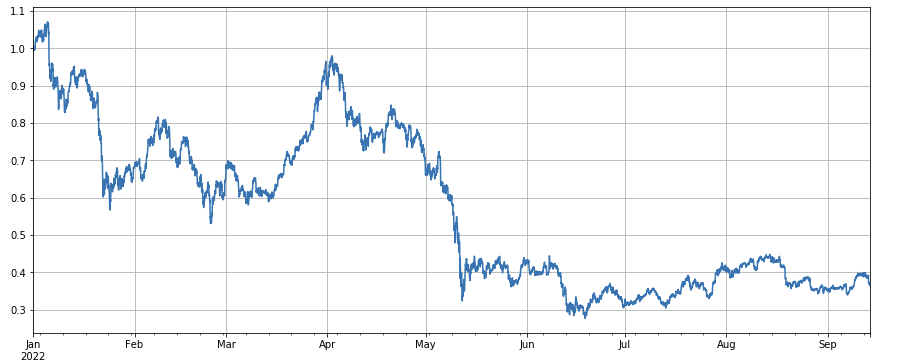
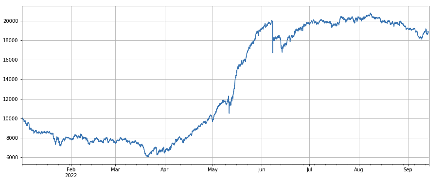
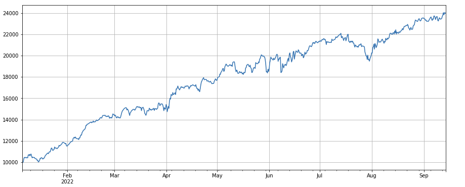
The overall performance of the market index is bleak, falling by 60% from the beginning of the year to recent days.

df_norm = df_close/df_close.fillna(method='bfill').iloc[0] #normalization
df_norm.mean(axis=1).plot(figsize=(15,6),grid=True);
#Final index profit chart

Factor validity judgment

• Regression method The yield of the following period is the dependent variable, and the factor to be tested is the independent variable. The coefficient obtained by regression is also the yield of the factor. After the regression equation is constructed, the validity and volatility of factors are generally viewed by reference to the absolute mean value of the coefficient t value, the proportion of the absolute value sequence of the coefficient t value greater than 2, the annualized factor return, the annualized factor profit volatility, and the Sharpe ratio of the factor profit. Multiple factors can be regressed at one time. Please refer to barra document for details.

• IC, IR and other indicators The so-called IC is the correlation coefficient between the factor and the return rate of the next period. Now, RANK_ IC is also used generally, it’s the correlation coefficient between factor ranking and the next stock return rate. IR is generally the mean value of IC sequence/the standard deviation of IC sequence.

• Stratified regression method In this paper, we will use this method, which is to sort the currencies according to the factors to be tested, divide them into N groups for group backtesting, and use a fixed period for position adjustment. If the situation is ideal, the return rate of Group N currencies will show a good monotony, increasing or decreasing monotonically, and the income gap of each group is large. Such factors are reflected in good discrimination. If the first group has the highest profits and the last group has the lowest profits, then go long in the first group and go short in the last group to get the final yield, which is the reference indicator of Sharp ratio.

Actual backtest operation

The coins to be selected are divided into 3 groups based on the ranking of the factors from smallest to largest. Each group of currencies accounts for about 1/3 of the total. If a factor is effective, the smaller the number of points in each group, the higher the return rate will be, but it also means that each currency has relatively more funds allocated. If the long and short positions are double leverage respectively, and the first group and the last group are 10 currencies respectively, then one currency accounts for 10% of the total. If a currency that is shorted is doubled, then 20% is withdrawn; If the number of groups is 50, then 4% will be withdrawn. Diversifying currencies can reduce the risk of black swans. Go long the first group (minimum factor value), go short the third group. The bigger the factor is, and the income will be higher, you can reverse the long and short position or simply turn the factor into a negative or reciprocal number.

Generally, the factor prediction ability can be roughly evaluated according to the return rate and Sharpe ratio of the final backtest. In addition, it also needs to refer to whether the factor expression is simple, sensitive to the size of the grouping, sensitive to the position adjustment interval, and sensitive to the initial time of the backtest.

With regard to the frequency of position adjustment, the stock market usually has a period of 5 days, 10 days and one month. However, for the digital currency market, such a period is undoubtedly too long, and the market in the real bot is monitored in real time. It is not necessary to stick to a specific period to adjust positions again. Therefore, in the real bot, we adjust positions in real time or in a short period of time.

As for how to close the position, according to the traditional method, the position can be closed if it is not in the group when sorting next time. However, in the case of real-time position adjustment, some currencies may be just at the boundary, which may lead to back and forth position closing. Therefore, this strategy adopts the method to wait for grouping changes, and then close the position when the position in the opposite direction needs to be opened. For example, the first group goes long. When the currencies in the long postion status are divided into the third group, then close the position and go short. If the position is closed in a fixed period, such as every day or every 8 hours, you can also close the position without being in a group. Try it more as you can.

#Backtest engine
class Exchange:
    
    def __init__(self, trade_symbols, fee=0.0004, initial_balance=10000):
        self.initial_balance = initial_balance #Initial assets
        self.fee = fee
        self.trade_symbols = trade_symbols
        self.account = {'USDT':{'realised_profit':0, 'unrealised_profit':0, 'total':initial_balance, 'fee':0, 'leverage':0, 'hold':0}}
        for symbol in trade_symbols:
            self.account[symbol] = {'amount':0, 'hold_price':0, 'value':0, 'price':0, 'realised_profit':0,'unrealised_profit':0,'fee':0}
            
    def Trade(self, symbol, direction, price, amount):
        
        cover_amount = 0 if direction*self.account[symbol]['amount'] >=0 else min(abs(self.account[symbol]['amount']), amount)
        open_amount = amount - cover_amount
        self.account['USDT']['realised_profit'] -= price*amount*self.fee #Net of fees
        self.account['USDT']['fee'] += price*amount*self.fee
        self.account[symbol]['fee'] += price*amount*self.fee

        if cover_amount > 0: #Close position first
            self.account['USDT']['realised_profit'] += -direction*(price - self.account[symbol]['hold_price'])*cover_amount  #Profits
            self.account[symbol]['realised_profit'] += -direction*(price - self.account[symbol]['hold_price'])*cover_amount
            
            self.account[symbol]['amount'] -= -direction*cover_amount
            self.account[symbol]['hold_price'] = 0 if self.account[symbol]['amount'] == 0 else self.account[symbol]['hold_price']
            
        if open_amount > 0:
            total_cost = self.account[symbol]['hold_price']*direction*self.account[symbol]['amount'] + price*open_amount
            total_amount = direction*self.account[symbol]['amount']+open_amount
            
            self.account[symbol]['hold_price'] = total_cost/total_amount
            self.account[symbol]['amount'] += direction*open_amount
                    
    
    def Buy(self, symbol, price, amount):
        self.Trade(symbol, 1, price, amount)
        
    def Sell(self, symbol, price, amount):
        self.Trade(symbol, -1, price, amount)
        
    def Update(self, close_price): #Update assets
        self.account['USDT']['unrealised_profit'] = 0
        self.account['USDT']['hold'] = 0
        for symbol in self.trade_symbols:
            if not np.isnan(close_price[symbol]):
                self.account[symbol]['unrealised_profit'] = (close_price[symbol] - self.account[symbol]['hold_price'])*self.account[symbol]['amount']
                self.account[symbol]['price'] = close_price[symbol]
                self.account[symbol]['value'] = abs(self.account[symbol]['amount'])*close_price[symbol]
                self.account['USDT']['hold'] += self.account[symbol]['value']
                self.account['USDT']['unrealised_profit'] += self.account[symbol]['unrealised_profit']
        self.account['USDT']['total'] = round(self.account['USDT']['realised_profit'] + self.initial_balance + self.account['USDT']['unrealised_profit'],6)
        self.account['USDT']['leverage'] = round(self.account['USDT']['hold']/self.account['USDT']['total'],3)

#Function of test factor
def Test(factor, symbols, period=1, N=40, value=300):
    e = Exchange(symbols, fee=0.0002, initial_balance=10000)
    res_list = []
    index_list = []
    factor = factor.dropna(how='all')
    for idx, row in factor.iterrows():
        if idx.hour % period == 0:
            buy_symbols =  row.sort_values().dropna()[0:N].index
            sell_symbols = row.sort_values().dropna()[-N:].index
            prices = df_close.loc[idx,]
            index_list.append(idx)
            for symbol in symbols:
                if symbol in buy_symbols and e.account[symbol]['amount'] <= 0:
                    e.Buy(symbol,prices[symbol],value/prices[symbol]-e.account[symbol]['amount'])
                if symbol in sell_symbols and e.account[symbol]['amount'] >= 0:
                    e.Sell(symbol,prices[symbol], value/prices[symbol]+e.account[symbol]['amount'])
            e.Update(prices)
            res_list.append([e.account['USDT']['total'],e.account['USDT']['hold']])
    return pd.DataFrame(data=res_list, columns=['total','hold'],index = index_list)

Simple factor test

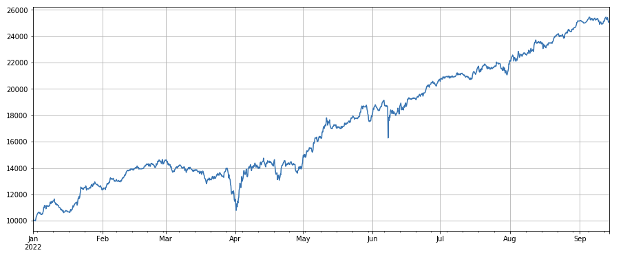
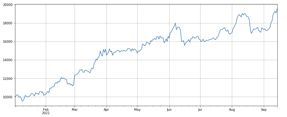
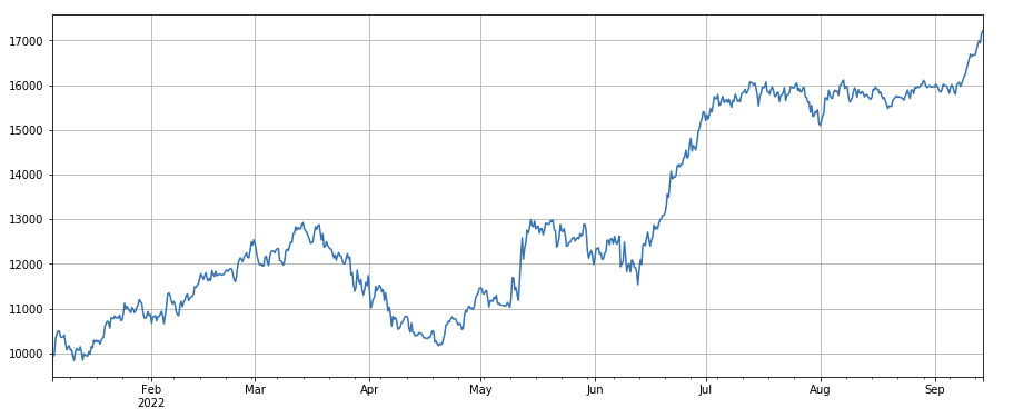
Trading volume factor: Simple long currencies with low trading volume and short currencies with high trading volume, which performs very well, indicating that popular currencies tend to decline.

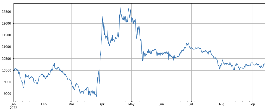
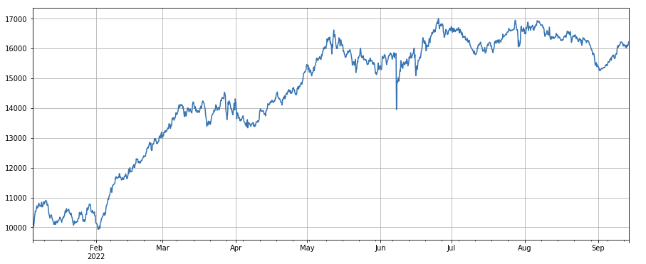
Trading price factor: the effect of going long currencies with low prices and going short currencies with high prices are both ordinary.

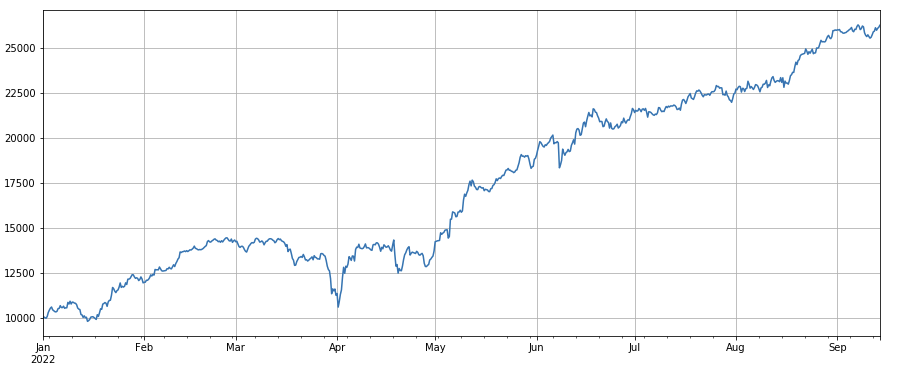
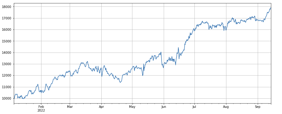
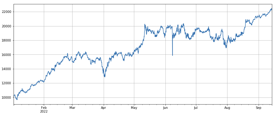
Transaction number factor: The performance is very similar to the transaction volume. It is obvious that the correlation between the transaction volume factor and the transaction number factor is very high. In fact, the average correlation between them in different currencies has reached 0.97, indicating that the two factors are very similar. This factor needs to be taken into account when synthesizing multiple factors.

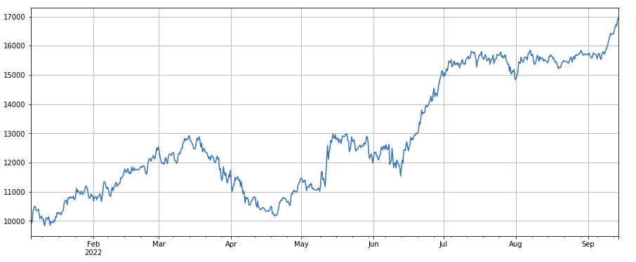
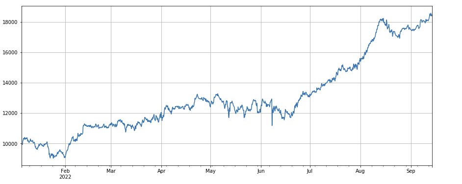
3h momentum factor: (df_close - df_close. shift (3))/df_ close. shift(3). That is, the 3-hour rise of the factor. The backtest results show that the 3-hour rise has obvious regression characteristics, that is, the rise is easier to fall later. The overall performance is OK, but there is also a long period of withdrawal and oscillation.

24h momentum factor: the result of 24h position adjustment period is good, the yield is similar to 3h momentum, and the withdraw is smaller.

Change factor of transaction volume: df_ volume.rolling(24).mean()/df_ volume. rolling (96). mean(), that is, the ratio of the transaction volume in the last day to the transaction volume in the last three days. The position is adjusted every 8h. The results of the backtesting were good, and the withdraw was also relatively low, indicating that those with active transaction volume were more inclined to decline.

Change factor of transaction number: df_ count.rolling(24).mean()/df_ count.rolling(96). mean (), that is, the ratio of the transaction number in the last day to the transaction number in the last three days. The position is adjusted every 8h. The results of the backtesting were good, and the withdraw is also relatively low, which indicates that those with active transaction volume were more inclined to decline.

Change factor of single transaction value: -(df_volume.rolling(24).mean()/df_count.rolling(24).mean())/(df_volume.rolling(24).mean()/df_count.rolling(96).mean()) , that is, the ratio of the transaction value of the last day to the transaction value of the last three days, and the position will be adjusted every 8h. This factor is also highly correlated with the transaction volume factor.

Change factor of taker by transaction proportion: df_buy_ratio.rolling(24).mean()/df_buy_ratio.rolling(96).mean(), that is, the ratio of the taker by volume to the total transaction volume in the last day to the transaction value in the last three days, and the position will be adjusted every 8 hours. This factor performs fairly well and it has little correlation with the transaction volume factor.

Volatility factor: (df_close/df_open).rolling(24).std(), go long currencies with low volatility, it has a certain effect.

Correlation factor between transaction volume and closing price: df_close.rolling(96).corr(df_volume), the closing price in the last four days has a correlation factor of transaction volume, which has performed well overall.

The factors listed here are based on the price volume. In fact, the combination of factor formulas can be very complex without obvious logic. You can refer to the famous ALPHA101 factor construction method: https://github.com/STHSF/alpha101.

#transaction volume
factor_volume = df_volume
factor_volume_res = Test(factor_volume, symbols, period=4)
factor_volume_res.total.plot(figsize=(15,6),grid=True);

#transaction price
factor_close = df_close
factor_close_res = Test(factor_close, symbols, period=8)
factor_close_res.total.plot(figsize=(15,6),grid=True);

#transaction count
factor_count = df_count
factor_count_res = Test(factor_count, symbols, period=8)
factor_count_res.total.plot(figsize=(15,6),grid=True);

print(df_count.corrwith(df_volume).mean())

0.9671246744996017

#3h momentum factor
factor_1 =  (df_close - df_close.shift(3))/df_close.shift(3)
factor_1_res = Test(factor_1,symbols,period=1)
factor_1_res.total.plot(figsize=(15,6),grid=True);

#24h momentum factor
factor_2 =  (df_close - df_close.shift(24))/df_close.shift(24)
factor_2_res = Test(factor_2,symbols,period=24)
tamenxuanfactor_2_res.total.plot(figsize=(15,6),grid=True);

#factor of transaction volume
factor_3 = df_volume.rolling(24).mean()/df_volume.rolling(96).mean()
factor_3_res = Test(factor_3, symbols, period=8)
factor_3_res.total.plot(figsize=(15,6),grid=True);

#factor of transaction number
factor_4 = df_count.rolling(24).mean()/df_count.rolling(96).mean()
factor_4_res = Test(factor_4, symbols, period=8)
factor_4_res.total.plot(figsize=(15,6),grid=True);

#factor correlation
print(factor_4.corrwith(factor_3).mean())

0.9707239580854841

#single transaction value factor
factor_5 = -(df_volume.rolling(24).mean()/df_count.rolling(24).mean())/(df_volume.rolling(24).mean()/df_count.rolling(96).mean())
factor_5_res = Test(factor_5, symbols, period=8)
factor_5_res.total.plot(figsize=(15,6),grid=True);

print(factor_4.corrwith(factor_5).mean())

0.861206620552479

#proportion factor of taker by transaction
factor_6 = df_buy_ratio.rolling(24).mean()/df_buy_ratio.rolling(96).mean()
factor_6_res = Test(factor_6, symbols, period=4)
factor_6_res.total.plot(figsize=(15,6),grid=True);

print(factor_3.corrwith(factor_6).mean())

0.1534572192503726

#volatility factor
factor_7 = (df_close/df_open).rolling(24).std()
factor_7_res = Test(factor_7, symbols, period=2)
factor_7_res.total.plot(figsize=(15,6),grid=True);

#correlation factor between transaction volume and closing price
factor_8 = df_close.rolling(96).corr(df_volume)
factor_8_res = Test(factor_8, symbols, period=4)
factor_8_res.total.plot(figsize=(15,6),grid=True);

Multifactor synthesis

It is certainly the most important part of the strategy construction process to discover new effective factors constantly, but without a good factor synthesis method, an excellent single alpha factor cannot play its maximum role. Common multi factor synthesis methods include:

Equal weight method: all factors to be synthesized are added with equal weights to obtain new factors after synthesis.

Weighting method of historical factor return rate: all factors to be combined are added according to the arithmetic mean of historical factor return rate in the latest period as the weight to obtain a new factor after synthesis. The factors that perform well in this method have higher weights.

Maximize IC_ IR weighting method: the average IC value of the composite factor over a period of history is used as the estimation of the IC value of the composite factor in the next period, and the covariance matrix of the historical IC value is used as the estimation of the volatility of the composite factor in the next period. According to IC_ IR is equal to the expected value of IC divided by the standard deviation of IC to obtain the optimal weight solution of the maximum composite factor IC_ IR.

Principal component analysis (PCA): PCA is a common method for data dimensionality reduction, and the correlation between factors may be high. The principal components after dimensionality reduction are used as synthetic factors.

This paper will reference the factor validity assignment manually. The methods described above can be referred to: ae933a8c-5a94-4d92-8f33-d92b70c36119.pdf

When testing single factors, the sorting is fixed, but multi factor synthesis needs to combine completely different data, so all factors need to be standardized, and the extreme value and missing value need to be removed generally. Here we use df_ volume\factor_ 1\factor_ 7\factor_ 6\factor_ 8 for synthesis.

#standardize functions, remove missing values and extreme values, and standardize
def norm_factor(factor):
    factor = factor.dropna(how='all')
    factor_clip = factor.apply(lambda x:x.clip(x.quantile(0.2), x.quantile(0.8)),axis=1)
    factor_norm = factor_clip.add(-factor_clip.mean(axis=1),axis ='index').div(factor_clip.std(axis=1),axis ='index')
    return factor_norm


df_volume_norm = norm_factor(df_volume)
factor_1_norm = norm_factor(factor_1)
factor_6_norm = norm_factor(factor_6)
factor_7_norm = norm_factor(factor_7)
factor_8_norm = norm_factor(factor_8)

factor_total = 0.6*df_volume_norm + 0.4*factor_1_norm + 0.2*factor_6_norm + 0.3*factor_7_norm + 0.4*factor_8_norm
factor_total_res = Test(factor_total, symbols, period=8)
factor_total_res.total.plot(figsize=(15,6),grid=True);

Summary

This paper introduces the test method of single factor and tests common single factors, and initially introduces the method of multi factor synthesis. However, there are many research contents of multi factor. Every point mentioned in the paper can be further developed. It is a feasible way to turn the research on various strategies into the exploration of alpha factor. The use of factor methodology can greatly speed up the verification of trading ideas, and there are many materials for reference.

The real bot from: https://www.fmz.com/robot/486605

Related

More