Modeling and Analysis of Bitcoin Volatility Based on ARMA-EGARCH Model
 0
1076
0
1076
ED, and the process was omitted.
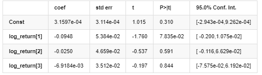
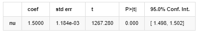
The matching degree of Normal normal distribution is not as good as t distribution, which also shows that the yield distribution has a thicker tail than the normal distribution. Next, enter the modeling process, an ARMA-GARCH(1,1) model regression is executed for log_return (logarithmic rate of return) and estimated as follows:
In [23]:
am_GARCH = arch_model(training_garch, mean='AR', vol='GARCH',
                      p=1, q=1, lags=3, dist='ged')
res_GARCH = am_GARCH.fit(disp=False, options={'ftol': 1e-01})
res_GARCH.summary()
Out[23]: Iteration: 1, Func. Count: 10, Neg. LLF: -1917.4262154917305
AR - GARCH Model Results
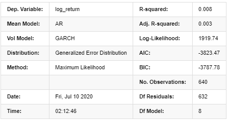
Mean Model
Volatility Model
Distribution
Covariance estimator: robust
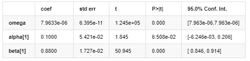
Description of GARCH volatility equation according to ARCH database:
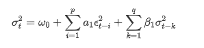
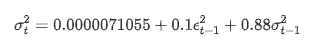
The conditional regression equation for volatility can be obtained as:
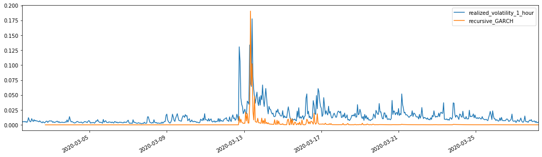
Combined with the matched predicted volatility, compare it with the realized volatility of the sample to see the effect.
In [26]:
def recursive_forecast(pd_dataframe):
    window = predict_lag
    model = 'GARCH'
    index = kline_test[1:].index
    end_loc = np.where(index >= kline_test.index[window])[0].min()
    forecasts = {}
    for i in range(len(kline_test[1:]) - window + 2):
        mod = arch_model(pd_dataframe['log_return'][1:], mean='AR', vol=model, dist='ged',p=1, q=1)
        res = mod.fit(last_obs=i+end_loc, disp='off', options={'ftol': 1e03})
        temp = res.forecast().variance
        fcast = temp.iloc[i + end_loc - 1]
        forecasts[fcast.name] = fcast

    forecasts = pd.DataFrame(forecasts).T
    pd_dataframe['recursive_{}'.format(model)] = forecasts['h.1']
    evaluate(pd_dataframe, 'realized_volatility_1_hour', 'recursive_{}'.format(model))

recursive_forecast(kline_test)
Out[26]: Mean Absolute Error (MAE): 0.0128 Mean Absolute Percentage Error (MAPE): 95.6 Root Mean Square Error (RMSE): 0.018
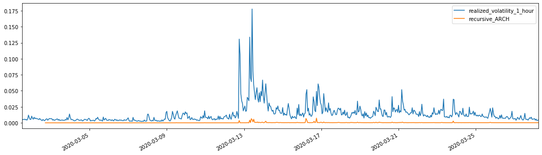
For comparison, make an ARCH as follows:
In [27]:
def recursive_forecast(pd_dataframe):
    window = predict_lag
    model = 'ARCH'
    index = kline_test[1:].index
    end_loc = np.where(index >= kline_test.index[window])[0].min()
    forecasts = {}
    for i in range(len(kline_test[1:]) - window + 2):
        mod = arch_model(pd_dataframe['log_return'][1:], mean='AR', vol=model, dist='ged', p=1)
        res = mod.fit(last_obs=i+end_loc, disp='off', options={'ftol': 1e03})
        temp = res.forecast().variance
        fcast = temp.iloc[i + end_loc - 1]
        forecasts[fcast.name] = fcast

    forecasts = pd.DataFrame(forecasts).T
    pd_dataframe['recursive_{}'.format(model)] = forecasts['h.1']
    evaluate(pd_dataframe, 'realized_volatility_1_hour', 'recursive_{}'.format(model))

recursive_forecast(kline_test)
Out[27]: Mean Absolute Error (MAE): 0.0136 Mean Absolute Percentage Error (MAPE): 98.1 Root Mean Square Error (RMSE): 0.02
7. EGARCH modeling
The next step is to perform EGARCH modeling
In [24]:
am_EGARCH = arch_model(training_egarch, mean='AR', vol='EGARCH',
                       p=1, lags=3, o=1,q=1, dist='ged')
res_EGARCH = am_EGARCH.fit(disp=False, options={'ftol': 1e-01})
res_EGARCH.summary()
Out[24]: Iteration: 1, Func. Count: 11, Neg. LLF: -1966.610328148909
AR - EGARCH Model Results
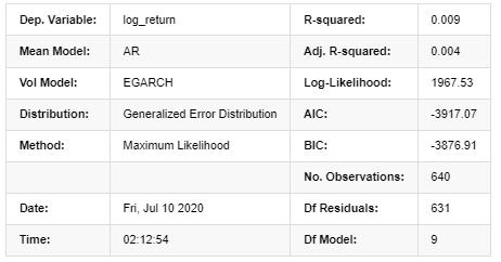
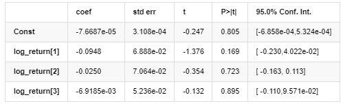
Mean Model
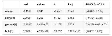
Volatility Model
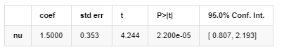
Distribution
Covariance estimator: robust
The EGARCH volatility equation provided by ARCH library is described as follows:
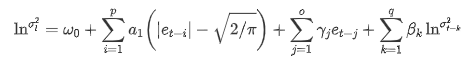
substitute
The conditional regression equation of volatility can be obtained as follows:

Among them, the estimated coefficient of symmetric term γ is less than the confidence interval, indicating that there is a significant “asymmetry” in the volatility of Bitcoin return rates.
Combined with the matched predicted volatility, the results are compared with the realized volatility of the sample as follows:
In [28]:
def recursive_forecast(pd_dataframe):
    window = 280
    model = 'EGARCH'
    index = kline_test[1:].index
    end_loc = np.where(index >= kline_test.index[window])[0].min()
    forecasts = {}
    for i in range(len(kline_test[1:]) - window + 2):
        mod = arch_model(pd_dataframe['log_return'][1:], mean='AR', vol=model,
                         lags=3, p=2, o=0, q=1, dist='ged')
        res = mod.fit(last_obs=i+end_loc, disp='off', options={'ftol': 1e03})
        temp = res.forecast().variance
        fcast = temp.iloc[i + end_loc - 1]
        forecasts[fcast.name] = fcast

    forecasts = pd.DataFrame(forecasts).T
    pd_dataframe['recursive_{}'.format(model)] = forecasts['h.1']
    evaluate(pd_dataframe, 'realized_volatility_1_hour', 'recursive_{}'.format(model))
    pd_dataframe['recursive_{}'.format(model)]

recursive_forecast(kline_test)
Out[28]: Mean Absolute Error (MAE): 0.0201 Mean Absolute Percentage Error (MAPE): 122 Root Mean Square Error (RMSE): 0.0279
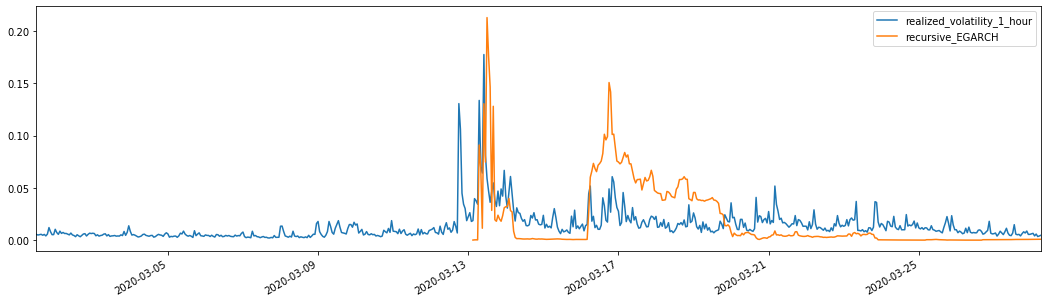
It can be seen that EGARCH is more sensitive to volatility and better matchs volatility than ARCH and GARCH.
8. Evaluation of volatility prediction
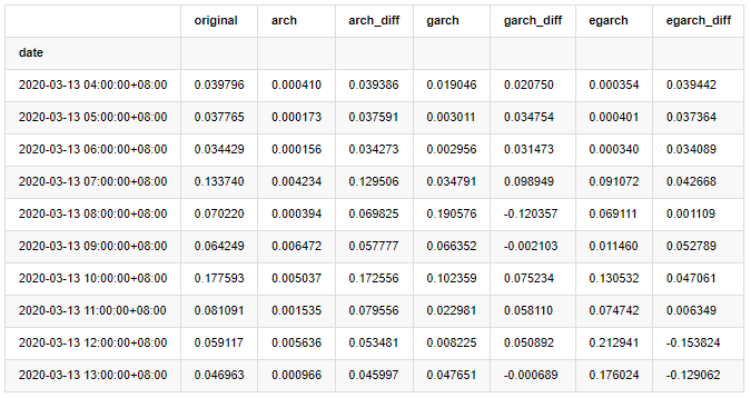
The hourly data is selected based on the sample, and the next step is to predict one hour ahead. We select the predicted volatility of the first 10 hours of the three models, with RV as the benchmark volatility. The comparative error value is as follows:
In [29]:
compare_ARCH_X = pd.DataFrame()
compare_ARCH_X['original']=kline_test['realized_volatility_1_hour']

compare_ARCH_X['arch']=kline_test['recursive_ARCH']
compare_ARCH_X['arch_diff']=compare_ARCH_X['original']-np.abs(compare_ARCH_X['arch'])

compare_ARCH_X['garch']=kline_test['recursive_GARCH']
compare_ARCH_X['garch_diff']=compare_ARCH_X['original']-np.abs(compare_ARCH_X['garch'])

compare_ARCH_X['egarch']=kline_test['recursive_EGARCH']
compare_ARCH_X['egarch_diff']=compare_ARCH_X['original']-np.abs(compare_ARCH_X['egarch'])
compare_ARCH_X = compare_ARCH_X[280:]
compare_ARCH_X.head(10)
Out[29]:
In [30]:
compare_ARCH_X_diff = pd.DataFrame(index=['ARCH','GARCH','EGARCH'], columns=['head 1 step', 'head 10 steps', 'head 100 steps'])
compare_ARCH_X_diff['head 1 step']['ARCH'] = compare_ARCH_X['arch_diff']['2020-03-13 04:00:00+08:00']
compare_ARCH_X_diff['head 10 steps']['ARCH'] = np.mean(compare_ARCH_X['arch_diff'][:10])
compare_ARCH_X_diff['head 100 steps']['ARCH'] = np.mean(compare_ARCH_X['arch_diff'][:100])
compare_ARCH_X_diff['head 1 step']['GARCH'] = compare_ARCH_X['garch_diff']['2020-03-13 04:00:00+08:00']
compare_ARCH_X_diff['head 10 steps']['GARCH'] = np.mean(compare_ARCH_X['garch_diff'][:10])
compare_ARCH_X_diff['head 100 steps']['GARCH'] = np.mean(compare_ARCH_X['garch_diff'][:100])
compare_ARCH_X_diff['head 1 step']['EGARCH'] = compare_ARCH_X['egarch_diff']['2020-03-13 04:00:00+08:00']
compare_ARCH_X_diff['head 10 steps']['EGARCH'] = np.mean(compare_ARCH_X['egarch_diff'][:10])
compare_ARCH_X_diff['head 100 steps']['EGARCH'] = np.abs(np.mean(compare_ARCH_X['egarch_diff'][:100]))
compare_ARCH_X_diff
Out[30]:
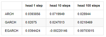
Several tests have been conducted, in the prediction results of the first hour, the probability of the smallest error of EGARCH is relatively large, but the overall difference is not particularly obvious; There are some obvious differences in short-term prediction effects; EGARCH has the most outstanding prediction ability in the long-term prediction
In [31]:
compare_ARCH_X = pd.DataFrame()
compare_ARCH_X['Model'] = ['ARCH','GARCH','EGARCH']
compare_ARCH_X['RMSE'] = [get_rmse(kline_test['realized_volatility_1_hour'][280:320],kline_test['recursive_ARCH'][280:320]),
                          get_rmse(kline_test['realized_volatility_1_hour'][280:320],kline_test['recursive_GARCH'][280:320]),
                          get_rmse(kline_test['realized_volatility_1_hour'][280:320],kline_test['recursive_EGARCH'][280:320])]
compare_ARCH_X['MAPE'] = [get_mape(kline_test['realized_volatility_1_hour'][280:320],kline_test['recursive_ARCH'][280:320]),
                          get_mape(kline_test['realized_volatility_1_hour'][280:320],kline_test['recursive_GARCH'][280:320]),
                          get_mape(kline_test['realized_volatility_1_hour'][280:320],kline_test['recursive_EGARCH'][280:320])]
compare_ARCH_X['MASE'] = [get_mape(kline_test['realized_volatility_1_hour'][280:320],kline_test['recursive_ARCH'][280:320]),
                          get_mape(kline_test['realized_volatility_1_hour'][280:320],kline_test['recursive_GARCH'][280:320]),
                          get_mape(kline_test['realized_volatility_1_hour'][280:320],kline_test['recursive_EGARCH'][280:320])]

compare_ARCH_X
Out[31]:
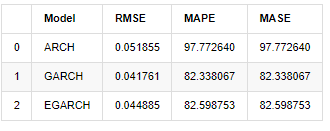
In terms of indicators, GARCH and EGARCH have some improvement compared with ARCH, but the difference is not particularly obvious. After multi sample interval selection and verification, EGARCH will have better performance, which is mainly because EGARCH explains the heteroscedasticity of samples well.
9. Conclusion
From the above simple analysis, it can be found that the logarithmic return rate of Bitcoin does not conform to the normal distribution, which is characterized by thick fat tails, and the volatility has aggregation and leverage effect, while showing obvious conditional heterogeneity.
In the prediction and evaluation of logarithmic rate of return, the ARMA model’s intra sample static prediction ability is better than the dynamic one significantly, which shows that the rolling method is obviously better than the iterative method, and can avoid the problems of overmatching and error amplification. The rate of return outside the sample is difficult to predict, which satisfies the weak efficiency assumption of the market.
In addition, when dealing with the thick tail phenomenon of Bitcoin, that is, the thick tail distribution of returns, it is found that the GED (generalized error) distribution is better than the t distribution and normal distribution significantly, which can improve the measurement accuracy of tail risk. At the same time, EGARCH has more advantages in predicting long-term volatility, which well explains the heteroscedasticity of the sample. The symmetric estimation coefficient in the model matching is less than the confidence interval, which indicates that there is a significant “asymmetry” in the return rates fluctuation of Bitcoin.
The whole modeling process is full of various bold assumptions, and there is no consistency identification depending on validity, so we can only verify some phenomena carefully. History can only support the probability of predicting the future in statistics, but the accuracy and cost performance ratio still have a long hard journey to go.
Compared with traditional markets, the availability of high-frequency data of Bitcoin is easier. The “realized” measurement of various indicators based on high-frequency data becomes simple and important. If nonparametric measures can provide quick observation for the market that has occurred, and measures with parameters can improve the input accuracy of the model, then taking the realized nonparametric measures as the “Hyperparameters” of the model may establish a more “complete” model.
However, the above is limited to theory. Higher frequency data can indeed provide more accurate analysis of traders’ behavior. It can not only provide more reliable tests for financial theoretical models, but also provide more abundant decision-making information for traders, even support the prediction of information flow and capital flow, and assist in designing more precise quantitative trading strategies. However, the Bitcoin market is so volatile that too long historical data can not match effective decision-making information, so high-frequency data will certainly bring greater market advantages to investors of digital currency.
Finally, if you think the above content helpful, you can also offer a little BTC to buy me a cup of Cola. But I don’t need coffee, I will fall asleep after drinking it····
- Example of Python MACD drawing
- Dynamic Balance Strategy Based on the Digital Currency
- SuperTrend V.1 -- Super Trend Line System
- Some Thoughts on the Logic of Digital Currency Futures Trading
- High frequency backtesting system based on transaction by transaction and defects of K-line backtesting
- 另一种TradingView信号执行策略方案
- What You Need to Know to Familiar with MyLanguage on FMZ -- Parameters of MyLanguage Trading Class Library
- What You Need to Know to Familiar with MyLanguage on FMZ -- Interface Charts
- Take you to analyze the Sharpe ratio, maximum drawdown, return rate and other indicator algorithms in the strategy backtesting
- 带您剖析策略回测中的夏普率、最大回撤、收益率等指标算法
- [Binance Championship] Binance Delivery Contract Strategy 3 - Butterfly Hedging
- The Use of Servers in Quantitative Trading
- Solution to Get the http Request Message Sent by the Docker
- A brief explanation of why it is not feasible to achieve asset movement on OKEX through a contract hedging strategy
- Detailed Explanation of Futures Backhand Doubling Algorithm Strategy Notes
- Earn 80 Times in 5 Days, the Power of High-frequency Strategy
- Research and Example on the Maker Spots and Futures Hedging Strategy Design
- Building a Quantitative Database of FMZ with SQLite
- How to Assign Different Version Data to a Rented Strategy via Strategy Rental Code Metadata
- Interest Arbitrage of Binance Perpetual Funding Rate (Current Bull Market Annualized 100%)