Linear pending order flow strategy developed based on data playback function

Linear pending order flow strategy developed based on data playback function

Preface

It is often said that trading is an art, and art comes from inspiration. So today I’d like to share with you how to use the FMZ Quant data playback function to explore my trading inspiration.

Inspiration and market feeling of trading

What we usually call inspiration refers to the creative state that people produce in the process of thinking. For traders, our left hemisphere of our brain has completed the formulation of a series of rules such as strategy writing, capital allocation and parameter setting. The inspiration and market feeling of trading comes from the right hemisphere of the brain.

Many people have heard of the word “market feeling”, which is a kind of vague feeling, just like a déjà vu of what is happening at the moment. Although this sixth sense like intuition in trading is not reasoned and analyzed logically, the anticipation of the future trend of the market will prompt traders to make buying or selling decisions.

How to get inspiration

In the eyes of a layman, the market feeling is mysterious. It is a mysterious talent. With it, you can stand on the market. In fact, it is a summary of subjective trading experience by the brain. It is a vague prejudgment feeling realized through years of watching the market.

Although strictly speaking, inspiration is not exactly the same as the market feeling, we believe that after thousands of times of market refinement, we will have a deeper understanding of the market, and we will be able to develop strategies with ease. So if you want to acquire this talent and develop more trading strategies. Only through a large number of transactions, can we improve our trading system.

However, domestic commodity futures and stocks only have a few hours of trading time a day, so it would be overwhelming to improve one’s experience in watching the market, forming one’s own profit patterns and trading rules, and training one’s conditioned reflexes subconsciously from live trading only. In addition to paying a long time cost, most traders also bear the cost of capital losses. In order to solve this problem, the FMZ Quant developed the data playback function.

How to use data playback

The data playback function can be trained regardless of the trading hours of the exchange, and it supports a variety of commodity futures and digital currency varieties. The market can be played back manually or automatically, and the start and end time and playback speed of the historical market can be set freely. Compared with other software, K-line data playback mode is widely used, while FMZ Quant adopts the data playback mode at the Tick level, which is really close to the backtesting environment of real bot trading, and it reproduces the price volume data of the market, allowing traders to immerse themselves in the real world.

Open the FMZ Quant official website (fmz.com) to register and log in, and then click the Database in the Dashboard to display the data playback function page. There are four option boxes and one selection button. First, click the selection button to display only the varieties that support real bot playback, then select the varieties to be played back at the top left, then select the start and end time of the data in the next two option boxes, then select the time period of the data as real bot playback, and finally click the Go button at the far right to start the data playback function.

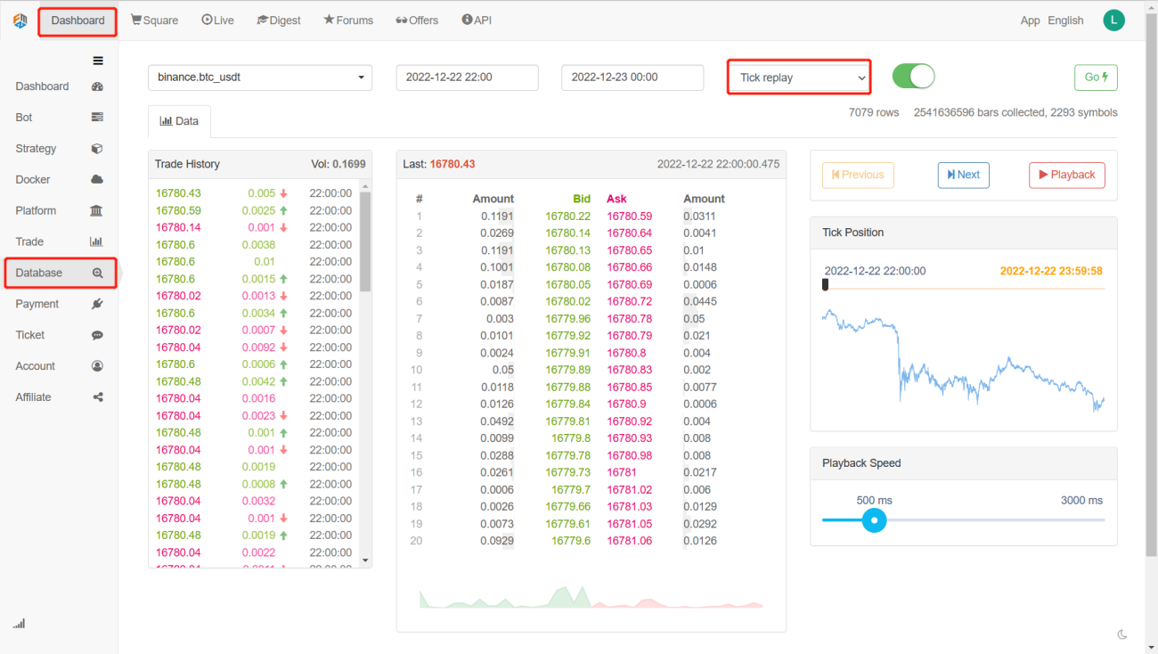
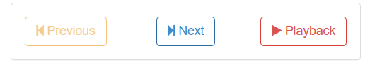
There are three sections under the data label. On the left is the trading history, where all the orders that have been closed are displayed in chronological order. In the middle is the 20-position depth of each buy and sell order data. On the right is the control area of data playback, where you can select manual and automatic data playback methods, just like using a media player.

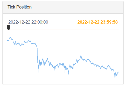
The position index can drag the cursor back and forth from left to right, allowing you to select the start time of data playback quickly.

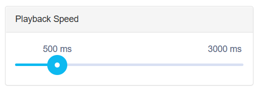
The speed of data playback can also be controlled at the bottom by moving the cursor right-left, in milliseconds, to both accelerate and decelerate the data during playback.

Build strategy logic

Although there are many factors that affect the price increasing and decreasing, including the global economic environment, national macro policies, relevant industrial policies, supply and demand relations, international events, interest rates and exchange rates, inflation and deflation, market psychology, unknown factors, etc., the final price on the market is the result of competition between various parties and the short position side. If more people buy than sell, the price will increase; On the contrary, if more people sell than buy, the price will decrease. Then we only need to analyze the price to make a trading strategy.

Through the FMZ Quant playback of the latest month’s BTC_USDT trading pairs of Binance exchange, we found that when the market increased and decreased sharply, the order book of Tick data is clearly asymmetric in terms of the volume of orders between the long and short positions. When the market is increasing, the number of going long orders is obviously greater than the number of going short orders; When the market is increasing, the number of going short orders is obviously greater than the number of going long orders. So can we predict the price increasing and decreasing in a short period of time based on the pending order volume in the order book?

The answer is yes.

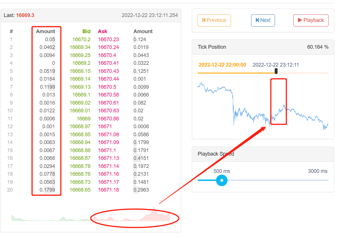
When the market is increasing, the number of going long orders is obviously greater than the number of going short orders.

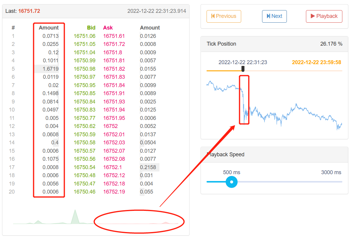
When the market is decreasing, the number of going short orders is obviously greater than the number of going long orders.

We can collect in-depth Tick data to calculate the long and short pending orders and compare them, if the combined long and short pending orders are very different, it may be a potential trading opportunity. For example, when the number of long position orders is N times that of short position orders, we can think that most people in the market are bullish, and the probability of price rise will increase in a short time in the future; When the number of short sellers is N times that of long sellers, we can think that most people in the market are bearish, and the probability of price decreasing will increase in the near future.

Write a trading strategy

According to the above strategy logic, it starts to be implemented in code. Open: fmz.com > Login > Dashboard > Strategy > Add Strategy > Click the drop-down menu in the upper right corner to select Python language and start writing strategies. This strategy serves as an introduction to teaching, so I try to simplify the strategy and pay attention to the comments in the following code.

Step 1: Write the strategy framework

# Strategy main function
def onTick():
    pass


# Program entry
def main():
    while True:  # Enter the infinite loop mode
        onTick()  # Execute the strategy main function
        Sleep(1000)  # Sleep for 1 second

We should write our strategy from big to small, just like building a house, building the frame first and then the wall. In this framework, we use two functions: the main function and the onTick function. The main function is the entry of the program, that is, the program will execute from here, then enter the infinite loop mode, and execute the onTick function repeatedly. Then we just need to write the strategy content into the onTick function.

Step 2: Write global variables

vol_ratio_arr = []  # Long/Short positions pending order ratio array
mp = 0  # Virtual positions

The reason why vol_ratio_arr is defined as a global variable, because my strategy needs to collect the ratio of long and short position pending orders of a piece of Tick data. If we put the vol_ratio_arr variable into the onTick function, it is obviously unreasonable to run with the loop. What we need is to change the value of the variable in the loop mode when a certain condition is met. The most reasonable way is to put the variable outside the loop.

Position management is very necessary, because it is related to the trading logic. Generally, we calculate the currency pairs held by acquiring accounts in spot transactions. In order to simplify the code, a global virtual position variable is directly defined to control the trading logic.

Step 3: Calculate the current multiple empty ratio

depth = exchange.GetDepth()  # Get depth data
asks = depth['Asks']  # Get asks array
bids = depth['Bids']  # Get bids array
asks_vol = 0  # All pending orders at ask price
bids_vol = 0  # All pending orders at bid price
for index, ask in enumerate(asks):  # Iterate through the ask price array
    # Linear calculation of all pending orders at the ask price
    asks_vol = asks_vol + ask['Amount'] * (20 - index)
for index, bid in enumerate(bids):  # Iterate through the bid price array
    # Linear calculation of all pending orders at the bid price
    bids_vol = bids_vol + bid['Amount'] * (20 - index)
bidask_ratio = bids_vol / asks_vol  # Calculate long/short position ratio

As we all know, digital currency is usually 20 levels of deep data, so we can add up the number of long and short position orders to calculate the ratio between long and short positions. When this value is greater than 1, it means that the bullish people are greater than the bearish people, indicating that the price will rise in a short period of time in the future; when this value is less than 1, it means that the bearish people are greater than the bullish people, indicating that the price will fall in a short period of time in the future.

However, there is a point to be distinguished. The closer the pending order is to the opening market, the stronger the desire to bullish or berish will be. For example, the order of the first level is definitely more willing to bullish than that of the 20th level. Therefore, when we accumulate the pending orders, we need to give different weights to the orders of the 20 levels in a linear way, which will be more reasonable.

Step 4: Linear calculation of the long/short position ratio in a period of time

global vol_ratio_arr, mp  # Introduce global variables
vol_ratio_arr.insert(0, bidask_ratio)  # Put the long/short position ratio into the global variable array
if len(vol_ratio_arr) > 20:  # If the array exceeds the specified length
    vol_ratio_arr.pop()  # Delete the oldest elements
all_ratio = 0  # Temporary variable, ratio of all long and short position pending orders
all_num = 0  # Temporary variables, all linear multipliers
for index, vol_ratio in enumerate(vol_ratio_arr):  # Variable global variable arrays
    num = 20 - index  # Linear multiplier
    all_num = all_num + num  # Linear multiplier accumulation
    all_ratio = all_ratio + vol_ratio * num  # Accumulation of all long and short position pending orders ratio
ratio = all_ratio / all_num  # Linear long and short position pending order ratio

The long-short position ratio can be obtained by dividing the long cumulative pending orders by the short cumulative pending orders. However, this is only a tick data. If only one tick data is used, it may not be a wise choice to decide buying and selling transactions, because in the rapidly changing market, one tick data is unconvincing. So we need to collect a fixed piece of Tick data, and finally calculate a fair value through linear calculation.

Step 5: Place an order

last_ask_price = asks[0]['Price']  # Latest buy one price for asks
last_bid_price = bids[0]['Price']  # Latest sell one price for bids
if mp == 0 and ratio > buy_threshold:  # If no currency is held currently, and the ratio is greater than the specified value
    exchange.Buy(last_ask_price, 0.01)  # Buy
    mp = 1  # Set the value of virtual position
if mp == 1 and ratio < sell_threshold:  # If there is currency held currently, and the ratio is less than the specified value
    exchange.Sell(last_bid_price, 0.01)  # Sell
    mp = 0  # Reset the value of virtual position

Because we need to specify a price when placing an order, we can directly use the latest sell one price when buying; When selling, you can directly use the latest buy one price. Finally, reset the value of virtual position after placing an order.

Conclusion

The above is the code analysis of the Linear pending order flow strategy developed based on data playback function. If you are a beginner of quantitative trading, the data playback function can learn trading at zero cost and shorten the time for understanding transactions. It usually takes several years for a real bot or simulated transaction to achieve initial results. It takes several weeks for the data playback function to achieve the same effect. On the premise of not wasting time, you can learn trading with minimal loss. For advanced traders, dynamic replay can help you analyze your past problems, verify and improve trading strategies, improve traders’ confidence in strategies, and help generate new strategic inspiration.