

Application of Machine Learning Technology in Trading
The inspiration of this article comes from my observation of some common warnings and traps after trying to apply machine learning technology to transaction problems during the data research on the FMZ Quant platform.
If you haven't read my previous articles, we suggest you read the automated data research environment guide and systematic method for formulating trading strategies that I established on the FMZ Quant platform before this article.
These two article addresses are here: https://www.fmz.com/digest-topic/9862 and https://www.fmz.com/digest-topic/9863.
About setting up the research environment
This tutorial is intended for enthusiasts, engineers and data scientists at all skill levels. Whether you are an industry leader or a programming novice, the only skills you need are a basic understanding of Python programming language and sufficient knowledge of command line operations (being able to set up a data science project is sufficient).
- Install the FMZ Quant docker and set up Anaconda
The FMZ Quant platform FMZ.COM not only provides high-quality data sources for major mainstream exchanges, but also provides a set of rich API interfaces to help us carry out automatic transactions after completing data analysis. This set of interfaces includes practical tools, such as querying account information, querying high, open, low, receipt price, trading volume, and various commonly used technical analysis indicators of various mainstream exchanges. In particular, it provides strong technical support for the public API interfaces connecting major mainstream exchanges in the actual trading process.
All the above mentioned features are encapsulated into a Docker-like system. What we need to do is to purchase or lease our own cloud computing services and deploy the Docker system.
In the official name of the FMZ Quant platform, the Docker system is called the Docker system.
Please refer to my previous article on how to deploy a docker and robot: https://www.fmz.com/bbs-topic/9864.
Readers who want to purchase their own cloud computing server to deploy dockers can refer to this article: https://www.fmz.com/digest-topic/5711.
After deploying the cloud computing server and the docker system successfully, next, we will install the present largest artifact of Python: Anaconda
In order to realize all the relevant program environments (dependency libraries, version management, etc.) required in this article, the simplest way is to use Anaconda. It is a packaged Python data science ecosystem and dependency library manager.
Since we install Anaconda on the cloud service, we recommend that the cloud server install the Linux system plus the command line version of Anaconda.
For the installation method of Anaconda, please refer to the official guide of Anaconda: https://www.anaconda.com/distribution/.
If you are an experienced Python programmer and if you feel that you do not need to use Anaconda, it is no problem at all. I will assume that you do not need help when installing the necessary dependent environment. You can skip this section directly.
Develop a trading strategy
The final output of a trading strategy should answer the following questions:
-
Direction: Determine if the asset is cheap, expensive or fair value.
-
Opening position conditions: If the asset is cheap or expensive, you should go long or go short.
-
Closing position trade: if the asset is reasonably priced and we have a position in the asset (previous buy or sell), should you close the position?
-
Price range: the price (or range) at which the position was opened.
-
Quantity: the quantity of money traded (e.g., the amount of digital currency or the number of lots of commodity futures).
Machine learning can be used to answer each of these questions, but for the rest of this article, we will focus on the first question, which is the direction of the trade.
Strategic approach
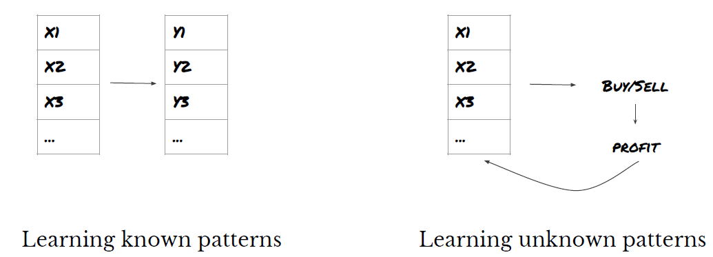
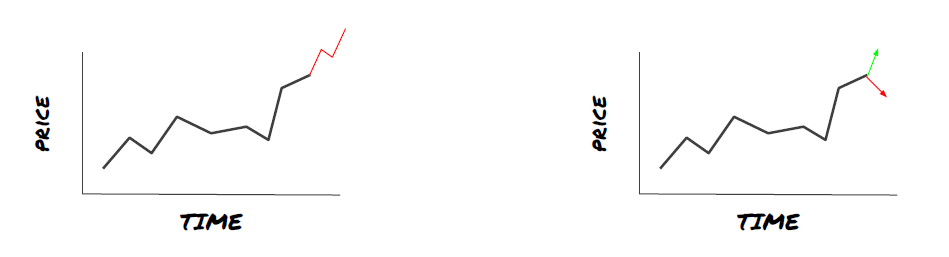
There are two types of approaches to constructing strategies: one is model-based; The other is based on data mining. These two methods are basically opposite to each other.
In the model-based strategy construction, we start from the market inefficiency model, build mathematical expressions (such as price and profit) and test their effectiveness in a long period of time. This model is usually a simplified version of a real complex model, and its long-term significance and stability need to be verified. The common trend following, mean reversion and arbitrage strategies fall into this category.
On the other hand, we look for price patterns first and try to use algorithms in data mining methods. The reasons for these patterns are not important, because only the identified patterns will continue to repeat in the future. This is a blind analysis method, and we need to check strictly to identify real patterns from random patterns. "Repeated test method", "k-line chart model" and "feature mass regression" belong to this category.
Obviously, machine learning is very easy to apply to data mining methods. Let's look at how to use machine learning to create transaction signals through data mining.
The code example uses a backtesting tool based on the FMZ Quant platform and an automated transaction API interface. After deploying the docker and installing Anaconda in the above section, you only need to install the data science analysis library we need and the famous machine learning model scikit-learn. We will not go over this section again.
pip install -U scikit-learn
Use machine learning to create trading strategy signals
-Data mining
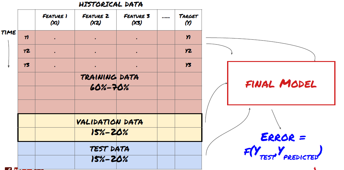
Before we begin, a standard machine learning problem system is shown in the following figure:
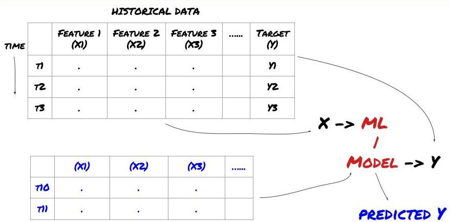
Machine learning problem system
The feature we are going to create must have some prediction ability (X). We want to predict the target variable (Y) and use historical data to train the ML model that can predict Y as close to the actual value as possible. Finally, we use this model to make predictions on new data where Y is unknown. This leads us to the first step:
Step 1: Set your question
- What do you want to predict? What is a good prediction? How do you evaluate the prediction results?
That is, in our framework above, what is Y?
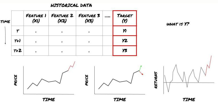
What do you want to predict?
Do you want to predict future prices, future returns/Pnl, buy/sell signals, optimize portfolio allocation and try to execute transactions efficiently?
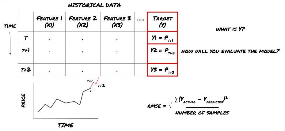
Suppose we try to forecast prices on the next timestamp. In this case, Y (t)=price (t+1). Now we can use historical data to complete our framework.
Note that Y (t) is known only in the backtest, but when we use our model, we will not know the price (t+1) of time t. We use our model to predict Y (predicted, t) and compare it with the actual value only at time t+1. This means that you cannot use Y as a feature in the prediction model.
Once we know the target Y, we can also decide how to evaluate our predictions. This is important to differentiate between the different models of the data we will try. Select an indicator to measure the efficiency of our model according to the problem we are solving. For example, if we predict prices, we can use root mean square error as an indicator. Some commonly used indicators (EMA, MACD, variance score, etc.) have been pre coded in the FMZ Quant toolbox. You can call these indicators globally through the API interface.
ML framework for predicting future prices
For demonstration purposes, we will create a prediction model to predict the expected future benchmark (basis) value of a hypothetical investment object, where:
            cpp

            basis = Price of Stock — Price of Future

basis(t)=S(t)−F(t)

Y(t) = future expected value of basis = Average(basis(t+1),basis(t+2),basis(t+3),basis(t+4),basis(t+5))
Since this is a regression problem, we will evaluate the model on RMSE (root mean square error). We will also use Total Pnl as the evaluation criteria.
Note: Please refer to Baidu Encyclopedia for relevant mathematical knowledge of RMSE.
- Our goal: to create a model to make the predicted value as close as possible to Y.
Step 2: Collect reliable data
Collect and clear data that can help you solve the problem at hand.
What data do you need to consider that can predict the target variable Y? If we predict the price, you can use the price data of the investment object, the trading quantity data of the investment object, the similar data of the related investment object, the index level of the investment object and other overall market indicators, and the price of other related assets.
You need to set data access permissions for these data and ensure that your data is accurate, and solve the lost data (a very common problem). At the same time, make sure that your data is impartial and fully representative of all market conditions (for example, the same number of profit and loss scenarios) to avoid bias in the model. You may also need to clean up the data to get dividends, split investment targets, continuations, etc.
If you use the FMZ Quant platform (FMZ. COM), we can access free global data from Google, Yahoo, NSE and Quandl; Depth data of domestic commodity futures such as CTP and Esunny; Data from mainstream digital currency exchanges such as Binance, OKX, Huobi and BitMex. The FMZ Quant platform also pre cleans and filters these data, such as the split of investment targets and in-depth market data, and presents them to strategy developers in a format that is easy for quantitative practitioners to understand.
To facilitate the demonstration of this article, we use the following data as the 'MQK' of the virtual investment target. We will also use a very convenient quantitative tool called Auquan's Toolbox. For more information, please refer to: https://github.com/Auquan/auquan-toolbox-python.
            python

            # Load the data
from backtester.dataSource.quant_quest_data_source import QuantQuestDataSource
cachedFolderName = '/Users/chandinijain/Auquan/qq2solver-data/historicalData/'
dataSetId = 'trainingData1'
instrumentIds = ['MQK']
ds = QuantQuestDataSource(cachedFolderName=cachedFolderName,
                                    dataSetId=dataSetId,
                                    instrumentIds=instrumentIds)
def loadData(ds):
    data = None
    for key in ds.getBookDataByFeature().keys():
        if data is None:
            data = pd.DataFrame(np.nan, index = ds.getBookDataByFeature()[key].index, columns=[])
        data[key] = ds.getBookDataByFeature()[key]
    data['Stock Price'] =  ds.getBookDataByFeature()['stockTopBidPrice'] + ds.getBookDataByFeature()['stockTopAskPrice'] / 2.0
    data['Future Price'] = ds.getBookDataByFeature()['futureTopBidPrice'] + ds.getBookDataByFeature()['futureTopAskPrice'] / 2.0
    data['Y(Target)'] = ds.getBookDataByFeature()['basis'].shift(-5)
    del data['benchmark_score']
    del data['FairValue']
    return data
data = loadData(ds)
With the above code, Auquan's Toolbox has downloaded and loaded the data into the data frame dictionary. We now need to prepare the data in the format we like. The function ds.getBookDataByFeature() returns the dictionary of data frames, one for each feature. We create new data frames for stocks with all characteristics.
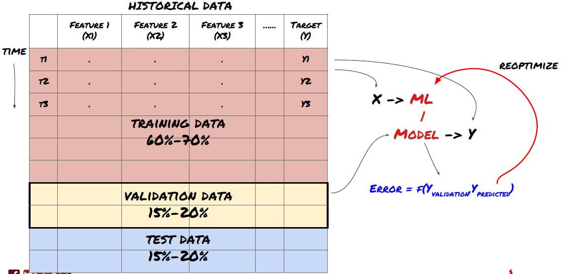
Step 3: Split the data
- Create training sets, cross verification and test these data sets from data.
This is a very important step! Before we continue, we should divide the data into training data sets to train your model; Test data sets to evaluate model performance. It is recommended to split them into 60-70% training sets and 30-40% test sets.
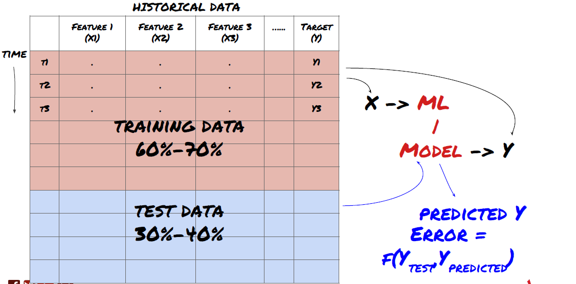
Split the data into training sets and test sets
Since training data is used to evaluate model parameters, your model may over fit these training data, and the training data may mislead model performance. If you do not retain any individual test data and use all the data for training, you will not know how well or badly your model performs on the new invisible data. This is one of the main reasons for the failure of the trained ML model in real-time data: people train all available data and are excited by the training data indicators, but the model cannot make any meaningful prediction on the untrained real-time data.
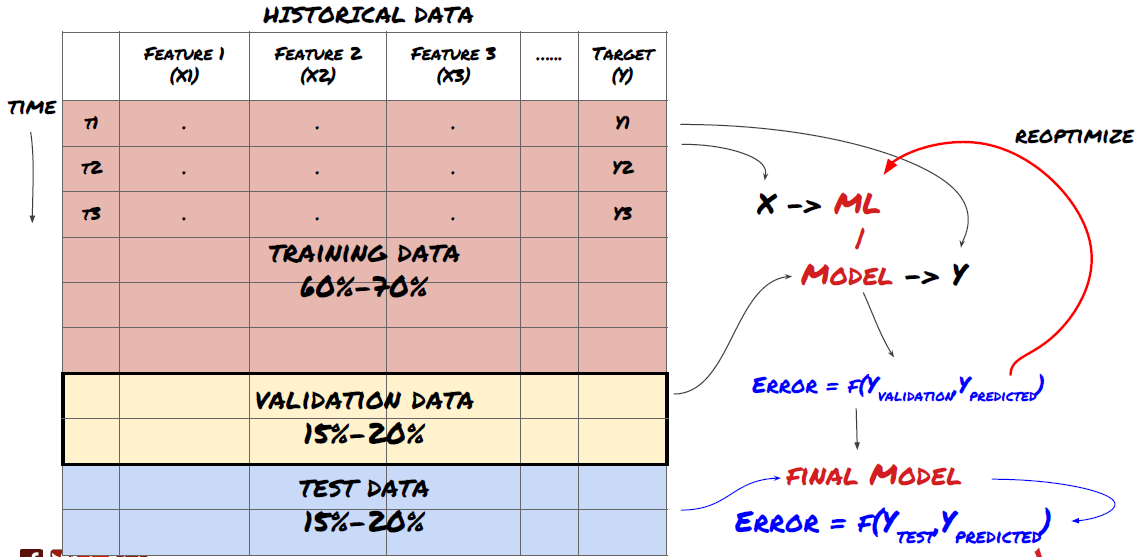
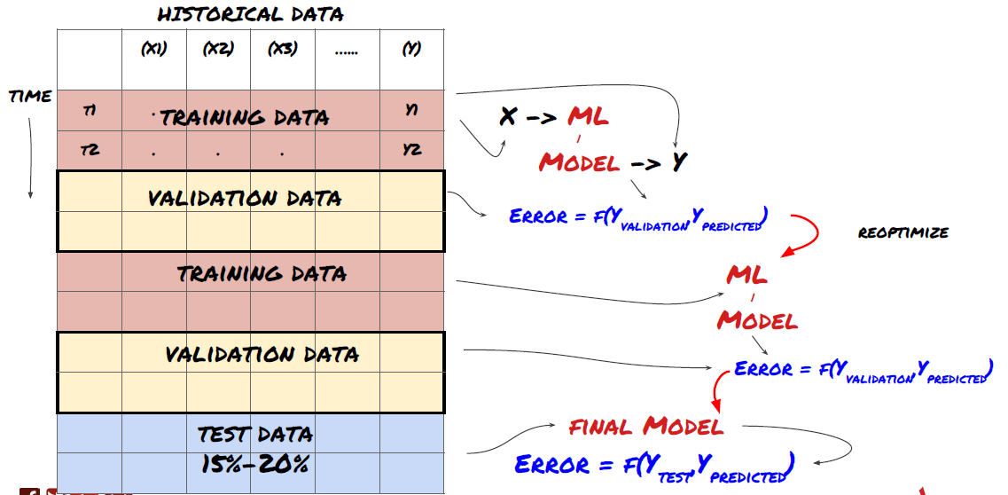
Split the data into training set, verification set and test set
There are problems with this method. If we train the training data repeatedly, evaluate the performance of the test data and optimize our model until we are satisfied with the performance, we take the test data as a part of the training data implicitly. In the end, our model may perform well on this set of training and test data, but it cannot guarantee that it can predict new data well.
To solve this problem, we can create a separate validation dataset. Now, you can train the data, evaluate the performance of the validation data, optimize until you are satisfied with the performance, and finally test the test data. In this way, the test data will not be polluted, and we will not use any information in the test data to improve our model.
Remember, once you have checked the performance of your test data, don't go back and try to further optimize your model. If you find that your model does not give good results, discard the model completely and start again. It is suggested that 60% of training data, 20% of validation data and 20% of test data can be split.
For our question, we have three available data sets. We will use one as the training set, the second as the verification set, and the third as our test set.
            python

            # Training Data
dataSetId =  'trainingData1'
ds_training = QuantQuestDataSource(cachedFolderName=cachedFolderName,
                                    dataSetId=dataSetId,
                                    instrumentIds=instrumentIds)
training_data = loadData(ds_training)
# Validation Data
dataSetId =  'trainingData2'
ds_validation = QuantQuestDataSource(cachedFolderName=cachedFolderName,
                                    dataSetId=dataSetId,
                                    instrumentIds=instrumentIds)
validation_data = loadData(ds_validation)
# Test Data
dataSetId =  'trainingData3'
ds_test = QuantQuestDataSource(cachedFolderName=cachedFolderName,
                                    dataSetId=dataSetId,
                                    instrumentIds=instrumentIds)
out_of_sample_test_data = loadData(ds_test)
For each of these, we add the target variable Y, which is defined as the average of the next five basis values.
            python

            def prepareData(data, period):
    data['Y(Target)'] = data['basis'].rolling(period).mean().shift(-period)
    if 'FairValue' in data.columns:
        del data['FairValue']
    data.dropna(inplace=True)
period = 5
prepareData(training_data, period)
prepareData(validation_data, period)
prepareData(out_of_sample_test_data, period)
Step 4: Feature engineering
Analyze data behavior and create predictive features
Now the real project construction has started. The golden rule of feature selection is that prediction ability mainly comes from features, not from models. You will find that the selection of features has a far greater impact on performance than the selection of models. Some considerations for feature selection:
-
Do not select a large set of features randomly without exploring the relationship with the target variable.
-
Little or no relationship with the target variable may lead to overfitting.
-
The features you select may be highly related to each other, in which case a small number of features can also explain the target.
-
I usually create some intuitive features, check the correlation between the target variable and these features, and the correlation between them to decide which one to use.
-
You can also try to perform principal component analysis (PCA) and other methods to sort candidate features according to the maximum information coefficient (MIC).
Feature transformation/normalization:
ML models tend to perform well in terms of normalization. However, normalization is difficult when dealing with time series data, because the future data range is unknown. Your data may be out of the normalization range, leading to model errors. But you can still try to force some degree of stability:
-
Scaling: dividing features by standard deviation or quartile range.
-
Centering: subtract the historical average value from the current value.
-
Normalization: two retrospective periods of the above (x - mean)/stdev.
-
Regular normalization: standardize the data into the range of - 1 to +1 and redetermine the center within the backtracking period (x-min)/(max min).
Note that since we use historical continuous average value, standard deviation, maximum or minimum values beyond the backtracking period, the normalized standardization value of the feature will represent different actual values at different times. For example, if the current value of the feature is 5 and the average value for 30 consecutive periods is 4.5, it will be converted to 0.5 after centering. After that, if the average value of 30 consecutive periods becomes 3, the value 3.5 will become 0.5. This may be the cause of the wrong model. Therefore, normalization is tricky, and you must figure out what improves the performance of the model actually (if any).
For the first iteration in our problem, we created a large number of features by using mixed parameters. Later we will try to see if we can reduce the number of features.
            python

            def difference(dataDf, period):
    return dataDf.sub(dataDf.shift(period), fill_value=0)
def ewm(dataDf, halflife):
    return dataDf.ewm(halflife=halflife, ignore_na=False,
                      min_periods=0, adjust=True).mean()
def rsi(data, period):
    data_upside = data.sub(data.shift(1), fill_value=0)
    data_downside = data_upside.copy()
    data_downside[data_upside > 0] = 0
    data_upside[data_upside < 0] = 0
    avg_upside = data_upside.rolling(period).mean()
    avg_downside = - data_downside.rolling(period).mean()
    rsi = 100 - (100 * avg_downside / (avg_downside + avg_upside))
    rsi[avg_downside == 0] = 100
    rsi[(avg_downside == 0) & (avg_upside == 0)] = 0
return rsi
def create_features(data):
    basis_X = pd.DataFrame(index = data.index, columns =  [])

    basis_X['mom3'] = difference(data['basis'],4)
    basis_X['mom5'] = difference(data['basis'],6)
    basis_X['mom10'] = difference(data['basis'],11)

    basis_X['rsi15'] = rsi(data['basis'],15)
    basis_X['rsi10'] = rsi(data['basis'],10)

    basis_X['emabasis3'] = ewm(data['basis'],3)
    basis_X['emabasis5'] = ewm(data['basis'],5)
    basis_X['emabasis7'] = ewm(data['basis'],7)
    basis_X['emabasis10'] = ewm(data['basis'],10)
    basis_X['basis'] = data['basis']
    basis_X['vwapbasis'] = data['stockVWAP']-data['futureVWAP']

    basis_X['swidth'] = data['stockTopAskPrice'] -
                        data['stockTopBidPrice']
    basis_X['fwidth'] = data['futureTopAskPrice'] -
                        data['futureTopBidPrice']

    basis_X['btopask'] = data['stockTopAskPrice'] -
                         data['futureTopAskPrice']
    basis_X['btopbid'] = data['stockTopBidPrice'] -
                         data['futureTopBidPrice']

    basis_X['totalaskvol'] = data['stockTotalAskVol'] -
                             data['futureTotalAskVol']
    basis_X['totalbidvol'] = data['stockTotalBidVol'] -
                             data['futureTotalBidVol']

    basis_X['emabasisdi7'] = basis_X['emabasis7'] -
                             basis_X['emabasis5'] +
                             basis_X['emabasis3']

    basis_X = basis_X.fillna(0)

    basis_y = data['Y(Target)']
    basis_y.dropna(inplace=True)

    print("Any null data in y: %s, X: %s"
            %(basis_y.isnull().values.any(),
             basis_X.isnull().values.any()))
    print("Length y: %s, X: %s"
            %(len(basis_y.index), len(basis_X.index)))

    return basis_X, basis_y
basis_X_train, basis_y_train = create_features(training_data)
basis_X_test, basis_y_test = create_features(validation_data)
Step 5: Model selection
Select the appropriate statistical/ML model according to the selected questions
The choice of model depends on how the problem is formed. Are you solving supervised (each point X in the feature matrix is mapped to the target variable Y) or unsupervised learning (without a given mapping, the model tries to learn an unknown pattern)? Are you dealing with regression (forecasting the actual price in the future time) or classification (only forecasting the price direction in the future time (increase/decrease))?
Supervised or unsupervised learning
Regression or classification
Some common supervised learning algorithms can help you get started:
-
Linear regression (parameters, regression)
-
Logistic regression (parameter, classification)
-
K-Nearest Neighbor (KNN) algorithm (case-based, regression)
-
SVM, SVR (parameters, classification and regression)
-
Decision tree
-
Decision forest
I suggest starting with a simple model, such as linear or logistic regression, and building more complex models from there as needed. It is also recommended that you read the mathematics behind the model rather than using it as a black box blindly.
Step 6: Training, verification and optimization (repeat steps 4-6)
Use training and verification data sets to train and optimize your model
Now you are ready to finally build the model. At this stage, you really just iterate the model and model parameters. Train your model on the training data, measure its performance on the verification data, and then return, optimize, retrain and evaluate it. If you are not satisfied with the performance of the model, please try another model. You cycle through this phase many times until you finally have a model that you are satisfied with.
Only when you have your favorite model, then move on to the next step.
For our demonstration problem, let's start with a simple linear regression:
python
from sklearn import linear_model
from sklearn.metrics import mean_squared_error, r2_score
def linear_regression(basis_X_train, basis_y_train,
basis_X_test,basis_y_test):
regr = linear_model.LinearRegression()
# Train the model using the training sets
regr.fit(basis_X_train, basis_y_train)
# Make predictions using the testing set
basis_y_pred = regr.predict(basis_X_test)
# The coefficients
print('Coefficients: \n', regr.coef_)
# The mean squared error
print("Mean squared error: %.2f"
% mean_squared_error(basis_y_test, basis_y_pred))
# Explained variance score: 1 is perfect prediction
print('Variance score: %.2f' % r2_score(basis_y_test,
basis_y_pred))
# Plot outputs
plt.scatter(basis_y_pred, basis_y_test, color='black')
plt.plot(basis_y_test, basis_y_test, color='blue', linewidth=3)
plt.xlabel('Y(actual)')
plt.ylabel('Y(Predicted)')
plt.show()
return regr, basis_y_pred
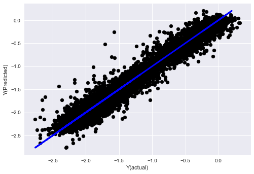
_, basis_y_pred = linear_regression(basis_X_train, basis_y_train,
basis_X_test,basis_y_test)
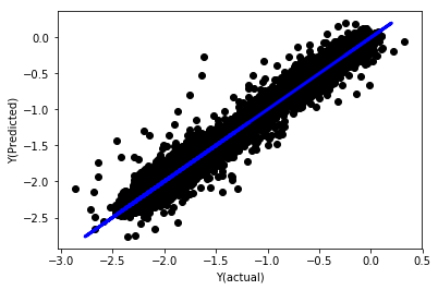
Linear regression without normalization
            mylang

            ('Coefficients: \n', array([ -1.0929e+08, 4.1621e+07, 1.4755e+07, 5.6988e+06, -5.656e+01, -6.18e-04, -8.2541e-05,4.3606e-02, -3.0647e-02, 1.8826e+07, 8.3561e-02, 3.723e-03, -6.2637e-03, 1.8826e+07, 1.8826e+07, 6.4277e-02, 5.7254e-02, 3.3435e-03, 1.6376e-02, -7.3588e-03, -8.1531e-04, -3.9095e-02, 3.1418e-02, 3.3321e-03, -1.3262e-06, -1.3433e+07, 3.5821e+07, 2.6764e+07, -8.0394e+06, -2.2388e+06, -1.7096e+07]))
Mean squared error: 0.02
Variance score: 0.96
Look at the model coefficients. We can't really compare them or say which one is important, because they all belong to different scales. Let's try normalization to make them conform to the same proportion and also enforce some smoothness.
python
def normalize(basis_X, basis_y, period):
basis_X_norm = (basis_X - basis_X.rolling(period).mean())/
basis_X.rolling(period).std()
basis_X_norm.dropna(inplace=True)
basis_y_norm = (basis_y -
basis_X['basis'].rolling(period).mean())/
basis_X['basis'].rolling(period).std()
basis_y_norm = basis_y_norm[basis_X_norm.index]
return basis_X_norm, basis_y_norm
norm_period = 375
basis_X_norm_test, basis_y_norm_test = normalize(basis_X_test,basis_y_test, norm_period)
basis_X_norm_train, basis_y_norm_train = normalize(basis_X_train, basis_y_train, norm_period)
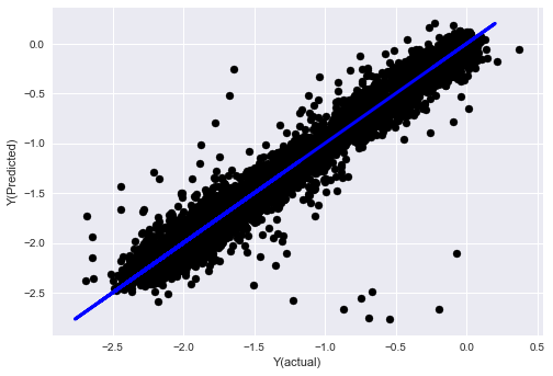
regr_norm, basis_y_pred = linear_regression(basis_X_norm_train, basis_y_norm_train, basis_X_norm_test, basis_y_norm_test)
basis_y_pred = basis_y_pred * basis_X_test['basis'].rolling(period).std()[basis_y_norm_test.index] + basis_X_test['basis'].rolling(period).mean()[basis_y_norm_test.index]
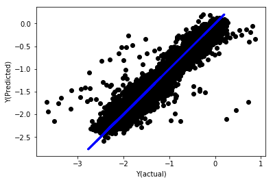
Linear regression with normalization
            mylang

            Mean squared error: 0.05
Variance score: 0.90
This model does not improve the previous model, but it is not worse. Now we can compare the coefficients to see which ones are important actually.
Let's look at the coefficients:
            python

            for i in range(len(basis_X_train.columns)):
    print('%.4f, %s'%(regr_norm.coef_[i], basis_X_train.columns[i]))
The results are:
            19.8727, emabasis4
-9.2015, emabasis5
8.8981, emabasis7
-5.5692, emabasis10
-0.0036, rsi15
-0.0146, rsi10
0.0196, mom10
-0.0035, mom5
-7.9138, basis
0.0062, swidth
0.0117, fwidth
2.0883, btopask
2.0311, btopbid
0.0974, bavgask
0.0611, bavgbid
0.0007, topaskvolratio
0.0113, topbidvolratio
-0.0220, totalaskvolratio
0.0231, totalbidvolratio
We can clearly see that some features have higher coefficients than others, and they may have stronger prediction ability.
Let's see the correlation between different features.
            python

            import seaborn

c = basis_X_train.corr()
plt.figure(figsize=(10,10))
seaborn.heatmap(c, cmap='RdYlGn_r', mask = (np.abs(c) <= 0.8))
plt.show()
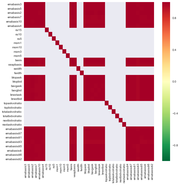
Correlation between features
The dark red areas represent highly correlated variables. Let's create/modify some features again and try to improve our model.
For example, I can discard features like emabasisdi7 easily, which are only linear combinations of other features.
python
def create_features_again(data):
basis_X = pd.DataFrame(index = data.index, columns = [])
basis_X['mom10'] = difference(data['basis'],11)
basis_X['emabasis2'] = ewm(data['basis'],2)
basis_X['emabasis5'] = ewm(data['basis'],5)
basis_X['emabasis10'] = ewm(data['basis'],10)
basis_X['basis'] = data['basis']
basis_X['totalaskvolratio'] = (data['stockTotalAskVol']
- data['futureTotalAskVol'])/
100000
basis_X['totalbidvolratio'] = (data['stockTotalBidVol']
- data['futureTotalBidVol'])/
100000
basis_X = basis_X.fillna(0)
basis_y = data['Y(Target)']
basis_y.dropna(inplace=True)
return basis_X, basis_y
basis_X_test, basis_y_test = create_features_again(validation_data)
basis_X_train, basis_y_train = create_features_again(training_data)
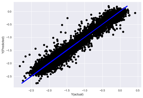
_, basis_y_pred = linear_regression(basis_X_train, basis_y_train, basis_X_test,basis_y_test)
basis_y_regr = basis_y_pred.copy()
            mylang

            ('Coefficients: ', array([ 0.03246139,
0.49780982, -0.22367172,  0.20275786,  0.50758852,
-0.21510795, 0.17153884]))
Mean squared error: 0.02
Variance score: 0.96
Look, the performance of our model has not changed. We only need some characteristics to explain our target variables. I suggest you try more of the above features, try new combinations, etc., to see what can improve our model.
We can also try more complex models to see whether changes in models can improve performance.
- K-Nearest Neighbor (KNN) algorithm
            javascript

            from sklearn import neighbors
n_neighbors = 5
model = neighbors.KNeighborsRegressor(n_neighbors, weights='distance')
model.fit(basis_X_train, basis_y_train)
basis_y_pred = model.predict(basis_X_test)
basis_y_knn = basis_y_pred.copy()
- SVR
            javascript

            from sklearn.svm import SVR
model = SVR(kernel='rbf', C=1e3, gamma=0.1)
model.fit(basis_X_train, basis_y_train)
basis_y_pred = model.predict(basis_X_test)
basis_y_svr = basis_y_pred.copy()
- Decision tree
            model=ensemble.ExtraTreesRegressor()
model.fit(basis_X_train, basis_y_train)
basis_y_pred = model.predict(basis_X_test)
basis_y_trees = basis_y_pred.copy()
Step 7: Backtest the test data
Check the performance of the actual sample data
Backtesting performance on (untouched) test data sets
This is a critical moment. We run our final optimization model from the last step of the test data, we put it aside at the beginning and we have not touched the data so far.
This gives you a realistic expectation of how your model will execute on new and unseen data when you start real-time trading. Therefore, it is necessary to ensure that you have a clean data set that is not used to train or verify the model.
If you do not like the backtest results of the test data, please discard the model and start again. Never go back or re-optimize your model, which will lead to over fitting! (It is also recommended to create a new test data set, because this data set is now polluted; when discarding the model, we already know the content of the data set implicitly).
Here we will still use Auquan's Toolbox:
            python

            import backtester
from backtester.features.feature import Feature
from backtester.trading_system import TradingSystem
from backtester.sample_scripts.fair_value_params import FairValueTradingParams
class Problem1Solver():
def getTrainingDataSet(self):
        return "trainingData1"
def getSymbolsToTrade(self):
        return ['MQK']
def getCustomFeatures(self):
        return {'my_custom_feature': MyCustomFeature}
def getFeatureConfigDicts(self):

        expma5dic = {'featureKey': 'emabasis5',
                 'featureId': 'exponential_moving_average',
                 'params': {'period': 5,
                              'featureName': 'basis'}}
        expma10dic = {'featureKey': 'emabasis10',
                 'featureId': 'exponential_moving_average',
                 'params': {'period': 10,
                              'featureName': 'basis'}}
        expma2dic = {'featureKey': 'emabasis3',
                 'featureId': 'exponential_moving_average',
                 'params': {'period': 3,
                              'featureName': 'basis'}}
        mom10dic = {'featureKey': 'mom10',
                 'featureId': 'difference',
                 'params': {'period': 11,
                              'featureName': 'basis'}}

        return [expma5dic,expma2dic,expma10dic,mom10dic]

    def getFairValue(self, updateNum, time, instrumentManager):
        # holder for all the instrument features
        lbInstF = instrumentManager.getlookbackInstrumentFeatures()
        mom10 = lbInstF.getFeatureDf('mom10').iloc[-1]
        emabasis2 = lbInstF.getFeatureDf('emabasis2').iloc[-1]
        emabasis5 = lbInstF.getFeatureDf('emabasis5').iloc[-1]
        emabasis10 = lbInstF.getFeatureDf('emabasis10').iloc[-1]
        basis = lbInstF.getFeatureDf('basis').iloc[-1]
        totalaskvol = lbInstF.getFeatureDf('stockTotalAskVol').iloc[-1] - lbInstF.getFeatureDf('futureTotalAskVol').iloc[-1]
        totalbidvol = lbInstF.getFeatureDf('stockTotalBidVol').iloc[-1] - lbInstF.getFeatureDf('futureTotalBidVol').iloc[-1]

        coeff = [ 0.03249183, 0.49675487, -0.22289464, 0.2025182, 0.5080227, -0.21557005, 0.17128488]
        newdf['MQK'] = coeff[0] * mom10['MQK'] + coeff[1] * emabasis2['MQK'] +\
                      coeff[2] * emabasis5['MQK'] + coeff[3] * emabasis10['MQK'] +\
                      coeff[4] * basis['MQK'] + coeff[5] * totalaskvol['MQK']+\
                      coeff[6] * totalbidvol['MQK']

        newdf.fillna(emabasis5,inplace=True)
        return newdf
problem1Solver = Problem1Solver()
tsParams = FairValueTradingParams(problem1Solver)
tradingSystem = TradingSystem(tsParams)
tradingSystem.startTrading(onlyAnalyze=False,
                           shouldPlot=True,
                           makeInstrumentCsvs=False)
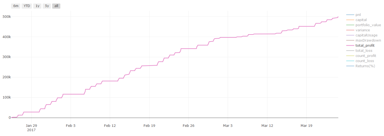
Backtesting results, Pnl is calculated in USD (Pnl is not included in transaction costs and other fees)
Step 8: Other methods to improve the model
Rolling verification, set learning, Bagging and Boosting
In addition to collecting more data, creating better features or trying more models, there are a few more points you can try to improve.
1. Rolling verification
Rolling verification
Market conditions rarely stay the same. Suppose you have a year's data, and you use the data from January to August for training, and use the data from September to December to test your model. You may train for a very specific set of market conditions eventually. Maybe there was no market fluctuation in the first half of the year, and some extreme news led to a sharp rise in the market in September. Your model will not be able to learn this model, and it will bring you garbage prediction results.
It may be better to try forward rolling verification, such as training from January to February, verification in March, retraining from April to May, verification in June, etc.
2. Set learning
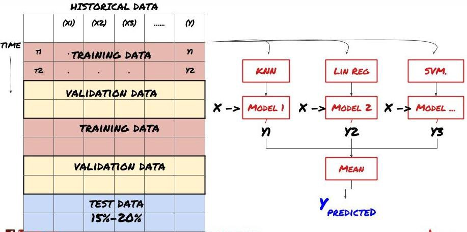
Set learning
Some models may be very effective in predicting certain scenarios, while models may be extremely overfitting in predicting other scenarios or under certain circumstances. One way to reduce errors and overfitting is to use a set of different models. Your prediction will be the average of the predictions made by many models, and the errors of different models may be offset or reduced. Some common set methods are Bagging and Boosting.
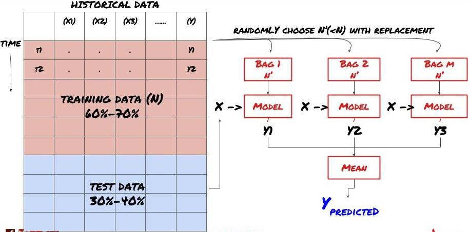
Bagging
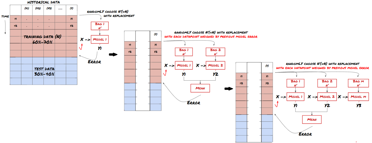
Boosting
For the sake of brevity, I'll skip these methods, but you can find more information online.
Let's try a set method for our problem:
            basis_y_pred_ensemble = (basis_y_trees + basis_y_svr +
                         basis_y_knn + basis_y_regr)/4
            mylang

            Mean squared error: 0.02
Variance score: 0.95
So far, we have accumulated a lot of knowledge and information. Let's review quickly:
-
Solve your problem;
-
Collect reliable data and clean up data;
-
Split data into training, verification and test sets;
-
Create features and analyze their behaviors;
-
Select appropriate training model according to the behavior;
-
Use training data to train your model and make predictions;
-
Check performance on verification set and re-optimize;
-
Verify the final performance of the test set.
Didn't that go to your heads? But it's not over yet. You only have a reliable prediction model. Remember what we really wanted in our strategy? So you don't need to:
-
Develop signals based on predictive models to identify trading directions;
-
Develop specific strategies to identify open and close positions;
-
Execute the system to identify positions and prices.
The above will use the FMZ Quant platform (FMZ.COM). On the FMZ Quant platform, there are highly encapsulated and perfect API interfaces, as well as ordering and trading functions that can be called globally. You don't need to connect and add API interfaces of different exchanges one by one. In the Strategy square of the FMZ Quant platform, there are many mature and perfect alternative strategies that match the machine learning method in this article, it will make your specific strategy more powerful. The strategy square is located at: https://www.fmz.com/square.
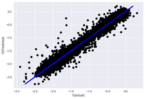
**Important note on transaction costs: ** Your model will tell you when the selected asset is going long or going short. However, it does not consider fees/transaction costs/available trading quantity/stop loss, etc. Transaction costs usually turn profitable transactions into losses. For example, an asset with an expected price increase of $0.05 is a buy, but if you have to pay $0.10 for this transaction, you will get a net loss of $0.05 eventually. After you take into account the broker's commission, exchange fee and point difference, our great profit chart above looks like this:
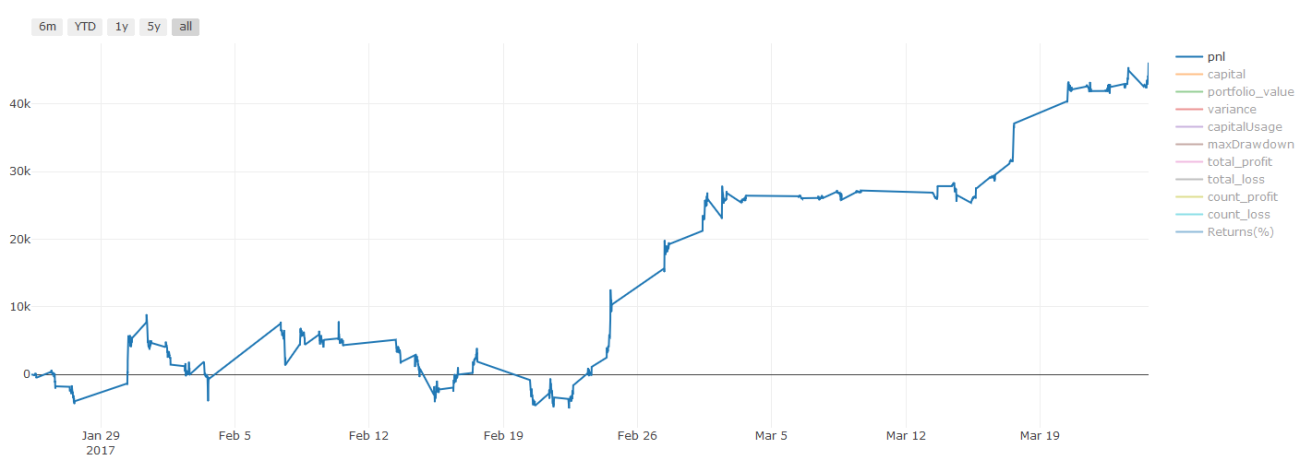
The backtest result after trading fees and point difference, Pnl is USD.
Transaction fees and price differences account for over 90% of our Pnl! We will discuss these in detail in a subsequent article.
Finally, let's take a look at some common pitfalls.
What to do and what not to do
-
Avoid over fitting with all your strength!
-
Don't retrain after every data point: this is a common mistake people make in machine learning development. If your model needs to be retrained after each data point, it may not be a very good model. That is to say, it needs to be retrained regularly, and only needs to be trained at a reasonable frequency (for example, if intra-day prediction is made, it needs to be retrained at the end of each week).
-
Avoid bias, especially forward-looking bias: This is another reason why the model does not work, and ensure that you do not use any future information. In most cases, this means that the target variable Y is not used as a feature in the model. You can use it during backtesting, but it will not be available when you run the model actually, which will make your model unusable.
-
Beware of data mining bias: As we are trying to conduct a series of modeling on our data to determine whether it is appropriate, if there is no special reason, please ensure that you run strict tests to separate the random mode from the actual mode that may occur. For example, linear regression explains the upward trend pattern well, but it is likely to become a fraction of the larger random wanderings!
Avoid over-fitting
This is very important. I think it is necessary to mention it again.
-
Overfitting is the most dangerous trap in trading strategies;
-
A complex algorithm may perform very well in the backtest, but it fails miserably on the new invisible data. This algorithm does not really reveal any trend of the data, nor does it have real prediction ability. It is very suitable for the data it sees;
-
Keep your system as simple as possible. If you find that you need a lot of complex functions to interpret data, you may overfit;
-
Divide your available data into training and test data, and always verify the performance of real sample data before using the model for real-time transactions.
- 1