

Quantitative Analysis of Digital Currency Market
A data-driven approach to speculative analysis of digital currencies
How about the price of Bitcoin? What are the reasons for the increasing and decreasing price of digital currency? Are the market prices of different Altcoins inextricably linked or largely independent? How can we predict what will happen next?
Articles about digital currency, such as Bitcoin and Ethereum, are now full of speculation. Hundreds of self-proclaimed experts are advocating the trend they expect. What many of these analyses lack is a solid foundation for basic data and statistical models.
The goal of this article is to provide a brief introduction to digital currency analysis by using Python. We will use a simple Python script to retrieve, analyze and visualize the data of different digital currencies. In this process, we will find interesting trends in the market behavior of these fluctuations and how they develop.
This is not an article explaining digital currency, nor is it an opinion about which specific currencies will increase and which will decrease. On the contrary, what we focus on in this tutorial is to obtain the original data and find the story hidden in the numbers.
Step 1: Set up our data working environment
This tutorial is intended for enthusiasts, engineers and data scientists at all skill levels. Whether you are an industry leader or a programming novice, the only skill you need is a basic understanding of Python programming language and sufficient knowledge of command line operations (being able to set up a data science project is sufficient).
1.1 Install the FMZ Quant docker and set up Anaconda
- Docker System of FMZ Quant platform
The FMZ Quant platform FMZ.COM not only provides high-quality data sources for major mainstream exchanges, but also provides a set of rich API interfaces to help us carry out automatic transactions after completing data analysis. This set of interfaces includes practical tools, such as querying account information, querying high, open, low, receipt price, trading volume, and various commonly used technical analysis indicators of various mainstream exchanges. In particular, it provides strong technical support for the public API interfaces connecting major mainstream exchanges in the actual trading process.
All the above-mentioned features are encapsulated into a Docker-like system. What we need to do is to purchase or lease our own cloud computing services and deploy the Docker system.
In the official name of the FMZ Quant platform, this Docker system is called the Docker system.
Please refer to my previous article on how to deploy a docker and robot: https://www.fmz.com/bbs-topic/9864.
Readers who want to purchase their own cloud computing server to deploy dockers can refer to this article: https://www.fmz.com/digest-topic/5711.
After deploying the cloud computing server and the docker system successfully, next, we will install the present largest artifact of Python: Anaconda
In order to realize all the relevant program environments (dependency libraries, version management, etc.) required in this article, the simplest way is to use Anaconda. It is a packaged Python data science ecosystem and dependency library manager.
Since we install Anaconda on the cloud service, we recommend that the cloud server install the Linux system plus the command line version of Anaconda.
For the installation method of Anaconda, please refer to the official guide of Anaconda: https://www.anaconda.com/distribution/.
If you are an experienced Python programmer and if you feel that you do not need to use Anaconda, it is no problem at all. I will assume that you do not need help when installing the necessary dependent environment. You can skip this section directly.
1.2 Create a data analysis project environment for Anaconda
Once Anaconda is installed, we need to create a new environment to manage our dependent packages. In the Linux command line interface, we input:
conda create --name cryptocurrency-analysis python=3
to create a new Anaconda environment for our project.
Next, input:
            python

            source activate cryptocurrency-analysis (linux/MacOS operating system)
or
activate cryptocurrency-analysis (windows operating system)
to activate the environment.
Next, input:
conda install numpy pandas nb_conda jupyter plotly
to install various dependent packages required for this project.
Note: Why use the Anaconda environment? If you plan to run many Python projects on your computer, it is helpful to separate the dependent packages (software libraries and packages) of different projects to avoid conflicts. Ananconda will create a special environment directory for the dependent packages of each project, so that all packages can be properly managed and distinguished.
1.3 Create a Jupyter Notebook
After the environment and dependent packages are installed, run:
jupyter notebook
to start the iPython kernel, then visit http://localhost:8888/ with your browser, create a new Python notebook, making sure it uses the:
Python [conda env:cryptocurrency-analysis]
kernel
1.4 Import dependent packages
Create an empty Jupyter notebook, and the first thing we need to do is import the required dependent packages.
            javascript

            import os
import numpy as np
import pandas as pd
import pickle
from datetime import datetime
We also need to import Plotly and enable offline mode:
            python

            import plotly.offline as py
import plotly.graph_objs as go
import plotly.figure_factory as ff
py.init_notebook_mode(connected=True)
Step 2: Get the price information of digital currency
The preparation is complete, and now we can start to obtain the data to be analyzed. First, we will use the API interface of the FMZ Quant platform to obtain the price data of Bitcoin.
This will use the GetTicker function. For the usage of these two functions, please refer to: https://www.fmz.com/api.
2.1 Write a Quandl data collection function
To facilitate data acquisition, we need to write a function to download and synchronize data from Quandl (quandl.com). This is a free financial data interface, which enjoys a high reputation abroad. The FMZ Quant platform also provides a similar data interface, which is mainly used for real bot transactions. Since the article mainly focuses on data analysis, we still use Quandl data here.
During the real bot transaction, you can call the GetTicker and GetRecords functions in Python directly to obtain price data. For their usage, please refer to: https://www.fmz.com/api.
            python

            def get_quandl_data(quandl_id):
    # Download and cache data columns from Quandl
    cache_path = '{}.pkl'.format(quandl_id).replace('/','-')
    try:
        f = open(cache_path, 'rb')
        df = pickle.load(f)
        print('Loaded {} from cache'.format(quandl_id))
    except (OSError, IOError) as e:
        print('Downloading {} from Quandl'.format(quandl_id))
        df = quandl.get(quandl_id, returns="pandas")
        df.to_pickle(cache_path)
        print('Cached {} at {}'.format(quandl_id, cache_path))
    return df
Here, the pickle library is used to serialize the data and save the downloaded data as a file, so that the program will not download the same data every time it runs. This function will return data in Pandas Dataframe format. If you are not familiar with the concept of data frame, you can imagine it as a powerful Excel.
2.2 Access to digital currency price data of Kraken exchange
Let's take the Kraken Bitcoin Exchange as an example, starting from obtaining its Bitcoin price.
            python

            # Get prices on the Kraken Bitcoin exchange
btc_usd_price_kraken = get_quandl_data('BCHARTS/KRAKENUSD')
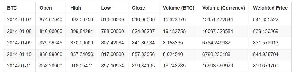
Use the head() method to view the first five rows of the data box.
btc_usd_price_kraken.head()
The result is:
Next, we are going to make a simple table in order to verify the correctness of the data by visualization.
            python

            # Make a table of BTC prices
btc_trace = go.Scatter(x=btc_usd_price_kraken.index, y=btc_usd_price_kraken['Weighted Price'])
py.iplot([btc_trace])
Here, we use Plotly to complete the visualization part. Compared with using some more mature Python data visualization libraries, such as Matplotlib, Plotly is a less common choice, but it is really a good choice, because it can call D3.js' fully interactive charts. These charts have beautiful default settings, which are easy to explore and very easy to embed into the web page.
Tips: The generated chart can be compared with the Bitcoin price chart of mainstream exchanges (such as the chart on OKX, Binance or Huobi) as a quick integrity check to confirm whether the downloaded data is generally consistent.
2.3 Obtain price data from mainstream Bitcoin exchanges
Careful readers may have noticed that there are missing data in the above data, especially at the end of 2014 and the beginning of 2016. Especially in Kraken Exchange, this kind of data loss is particularly obvious. We certainly do not hope that these missing data will affect the price analysis.
The characteristic of digital currency exchange is that the supply and demand relationship determines the currency price. Therefore, no transaction price can become the "mainstream price" of the market. In order to solve the problem and the data loss problem just mentioned (possibly due to technical power outages and data errors), we will download data from three mainstream Bitcoin exchanges in the world, and then calculate the average Bitcoin price.
Let's start by downloading the data of each exchange to the data frame composed of dictionary types.
            python

            # Download price data from COINBASE, BITSTAMP and ITBIT
exchanges = ['COINBASE','BITSTAMP','ITBIT']

exchange_data = {}

exchange_data['KRAKEN'] = btc_usd_price_kraken

for exchange in exchanges:
    exchange_code = 'BCHARTS/{}USD'.format(exchange)
    btc_exchange_df = get_quandl_data(exchange_code)
    exchange_data[exchange] = btc_exchange_df
2.4 Integrate all data into one data frame
Next, we will define a special function to merge the columns that are common to each data frame into a new data frame. Let's call it merge_dfs_on_column function.
            python

            def merge_dfs_on_column(dataframes, labels, col):
    '''Merge a single column of each dataframe into a new combined dataframe'''
    series_dict = {}
    for index in range(len(dataframes)):
        series_dict[labels[index]] = dataframes[index][col]

    return pd.DataFrame(series_dict)
Now, all data frames are integrated based on the "weighted price" column of each data set.
            python

            # Integrate all data frames
btc_usd_datasets = merge_dfs_on_column(list(exchange_data.values()), list(exchange_data.keys()), 'Weighted Price')
Finally, we use the "tail ()" method to view the last five rows of the merged data to ensure that the data is correct and complete.
btc_usd_datasets.tail()
The results are shown as:
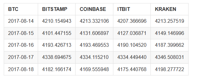
From the table above, we can see that these data are in line with our expectations, with roughly the same data range, but slightly different based on the delay or characteristics of each exchange.
2.5 Visualization process of price data
From the perspective of analysis logic, the next step is to compare these data through visualization. To do this, we need to define an auxiliary function first. By providing a single line command to use data to make a chart, we call it df_scatter function.
            python

            def df_scatter(df, title, seperate_y_axis=False, y_axis_label='', scale='linear', initial_hide=False):
    '''Generate a scatter plot of the entire dataframe'''
    label_arr = list(df)
    series_arr = list(map(lambda col: df[col], label_arr))

    layout = go.Layout(
        title=title,
        legend=dict(orientation="h"),
        xaxis=dict(type='date'),
        yaxis=dict(
            title=y_axis_label,
            showticklabels= not seperate_y_axis,
            type=scale
        )
    )

    y_axis_config = dict(
        overlaying='y',
        showticklabels=False,
        type=scale )

    visibility = 'visible'
    if initial_hide:
        visibility = 'legendonly'

    # Table tracking for each series
    trace_arr = []
    for index, series in enumerate(series_arr):
        trace = go.Scatter(
            x=series.index,
            y=series,
            name=label_arr[index],
            visible=visibility
        )

        # Add a separate axis to the series
        if seperate_y_axis:
            trace['yaxis'] = 'y{}'.format(index + 1)
            layout['yaxis{}'.format(index + 1)] = y_axis_config
        trace_arr.append(trace)

    fig = go.Figure(data=trace_arr, layout=layout)
    py.iplot(fig)
For your easy understanding, this article will not discuss the logic principle of this auxiliary function too much. If you want to know more, please check the official documentation of Pandas and Plotly.
Now, we can create Bitcoin price data charts easily!
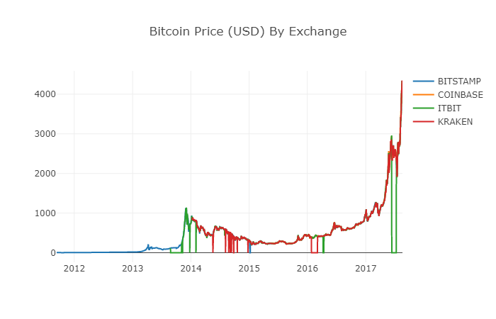
            python

            # Plot all BTC transaction prices
df_scatter(btc_usd_datasets, 'Bitcoin Price (USD) By Exchange')
2.6 Clear and aggregate price data
As can be seen from the chart above, although the four series of data follow roughly the same path, there are still some irregular changes. We will try to eliminate these irregular changes.
In the period of 2012-2017, we know that the price of Bitcoin has never been equal to zero, so we remove all zero values in the data frame first.
            python

            # Clear the "0" value
btc_usd_datasets.replace(0, np.nan, inplace=True)
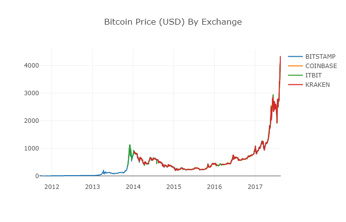
After reconstructing the data frames, we can see a clearer chart with no missing data anymore.
            python

            # Plot the revised data frame
df_scatter(btc_usd_datasets, 'Bitcoin Price (USD) By Exchange')
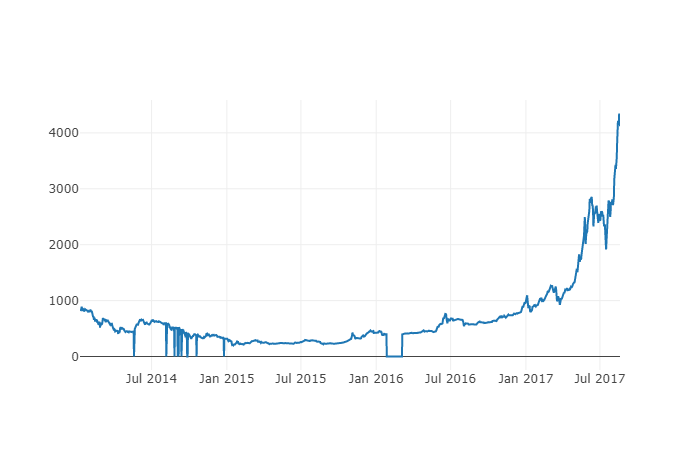
We can calculate a new column now: the daily average Bitcoin price of all exchanges.
            python

            # Calculate the average BTC price as a new column
btc_usd_datasets['avg_btc_price_usd'] = btc_usd_datasets.mean(axis=1)
The new column is the price index of Bitcoin! Let's draw it again to check whether the data looks wrong.
            python

            # Plot the average BTC price
btc_trace = go.Scatter(x=btc_usd_datasets.index, y=btc_usd_datasets['avg_btc_price_usd'])
py.iplot([btc_trace])
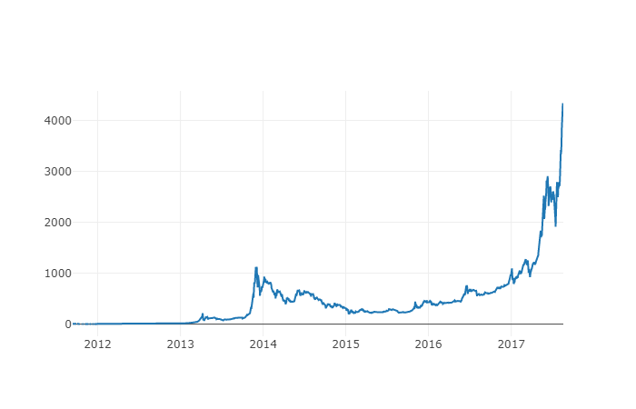
It seems that there is no problem. Later, we will continue to use this aggregated price series data to determine the exchange rate between other digital currencies and the USD.
Step 3: Collect the price of Altcoins
So far, we have the time series data of Bitcoin price. Next, let's take a look at some data of non-Bitcoin digital currencies, that is, Altcoins. Of course, the term "Altcoins" may be a bit hyperbole, but as far as the current development of digital currencies is concerned, except for the top ten in market value (such as Bitcoin, Ethereum, EOS, USDT, etc.), most of them can be called Altcoins. We should try to stay away from these currencies when trading, because they are too confusing and deceptive.
3.1 Define auxiliary functions through the API of the Poloniex exchange
First, we use the API of the Poloniex exchange to obtain the data information of digital currency transactions. We define two auxiliary functions to obtain the data related to Altcoins. These two functions mainly download and cache JSON data through APIs.
First, we define the function get_ json_data, which will download and cache JSON data from the given URL.
            python

            def get_json_data(json_url, cache_path):
    '''Download and cache JSON data, return as a dataframe.'''
    try:
        f = open(cache_path, 'rb')
        df = pickle.load(f)
        print('Loaded {} from cache'.format(json_url))
    except (OSError, IOError) as e:
        print('Downloading {}'.format(json_url))
        df = pd.read_json(json_url)
        df.to_pickle(cache_path)
        print('Cached {} at {}'.format(json_url, cache_path))
    return df
Next, we define a new function that will generate the HTTP request of the Poloniex API and call the just defined get_ json_data function to save the data results of the call.
python
base_polo_url = 'https://poloniex.com/public?command=returnChartData¤cyPair={}&start={}&end={}&period={}'
start_date = datetime.strptime('2015-01-01', '%Y-%m-%d') # Data acquisition since 2015
end_date = datetime.now() # Until today
pediod = 86400 # pull daily data (86,400 seconds per day)
def get_crypto_data(poloniex_pair):
'''Retrieve cryptocurrency data from poloniex'''
json_url = base_polo_url.format(poloniex_pair, start_date.timestamp(), end_date.timestamp(), pediod)
data_df = get_json_data(json_url, poloniex_pair)
data_df = data_df.set_index('date')
return data_df
The above function will extract the matching character code of digital currency (such as "BTC_ETH") and return the data frame containing the historical prices of two currencies.
3.2 Download transaction price data from Poloniex
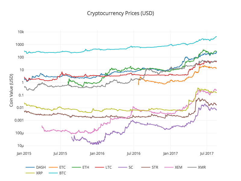
The vast majority of Altcoins cannot be purchased in USD directly. To obtain these digital currencies, individuals usually have to buy Bitcoin first, and then convert them into Altcoins according to their price ratio. Therefore, we have to download the exchange rate of each digital currency to Bitcoin, and then use the existing Bitcoin price data to convert it into USD. We will download the exchange rate data for the top 9 digital currencies: Ethereum, Litecoin, Ripple, EthereumClassic, Stellar, Dash, Siacoin, Monero, and NEM.
            python

            altcoins = ['ETH','LTC','XRP','ETC','STR','DASH','SC','XMR','XEM']

altcoin_data = {}
for altcoin in altcoins:
    coinpair = 'BTC_{}'.format(altcoin)
    crypto_price_df = get_crypto_data(coinpair)
    altcoin_data[altcoin] = crypto_price_df
Now, we have a dictionary containing 9 data frames, each of which contains historical daily average price data between Altcoins and Bitcoin.
We can determine whether the data is correct through the last few rows of the Ethereum price table.
            javascript

            altcoin_data['ETH'].tail()
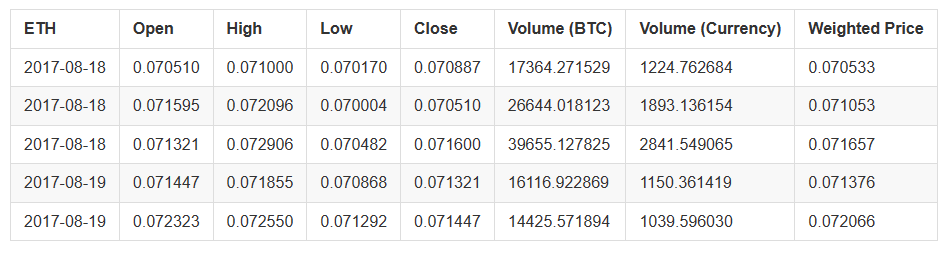
3.3 Unify the currency unit of all price data to USD
Now, we can combine BTC and Altcoins exchange rate data with our Bitcoin price index to calculate the historical price of each Altcoin (in USD) directly.
            python

            # Calculate USD Price as a new column in each altcoin data frame
for altcoin in altcoin_data.keys():
    altcoin_data[altcoin]['price_usd'] =  altcoin_data[altcoin]['weightedAverage'] * btc_usd_datasets['avg_btc_price_usd']
Here, we add a new column for each Altcoin data frame to store its corresponding USD price.
Next, we can reuse the function merge_dfs_on_column previously defined to create a combined data frame and integrate the USD price of each digital currency.
            python

            # Combine the USD price of each Altcoin into a single data frame
combined_df = merge_dfs_on_column(list(altcoin_data.values()), list(altcoin_data.keys()), 'price_usd')
Done!
Now let's add the Bitcoin price as the last column to the merged data frame.
            python

            # Add BTC price to data frame
combined_df['BTC'] = btc_usd_datasets['avg_btc_price_usd']
Now we have a unique data frame, which contains the daily USD prices of ten digital currencies that we are verifying.
We call the previous function df_scatter again, showing the corresponding prices of all Altcoins in the form of a chart.
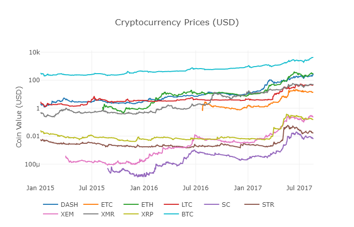
It seems that there is no problem in the chart. This chart shows us a complete picture of the change of the exchange price for each digital currency in the past few years.
Note: here we use the y-axis of logarithmic specification to compare all digital currencies on the same chart. You can also try different parameters (such as scale='linear') to understand data from different perspectives.
3.4 Start correlation analysis
Careful readers may have noticed that the prices of digital currencies seem to be relevant, although their currency values vary widely and are highly volatile. Especially since the rapid rise in April 2017, even many small fluctuations seem to occur simultaneously with the fluctuations of the whole market.
Of course, conclusions supported by data are more convincing than intuitions based on images.
We can use the Pandas corr() function to verify the above correlation hypothesis. This test method calculates the Pearson correlation coefficient of each column of the data frame corresponding to the other column.
Revision note on 2017.8.22: This section was modified to use the daily rate of return instead of the absolute value of the price when calculating the correlation coefficient.
Direct calculation based on a non-solid time series (such as raw price data) may lead to deviation of correlation coefficient. To solve this problem, our solution is to use the pct_change() method to convert the absolute value of each price in the data frame into the corresponding daily rate of return.
For example, let's calculate the correlation coefficient in 2016.
            python

            # Calculating the Pearson correlation coefficient for digital currencies in 2016
combined_df_2016 = combined_df[combined_df.index.year == 2016]
combined_df_2016.pct_change().corr(method='pearson')
The chart above shows the correlation coefficient. When the coefficient is close to 1 or - 1, it means that this series is positively correlated or negatively correlated, respectively. When the correlation coefficient is close to 0, it means that the corresponding objects are not correlated and their fluctuations are independent of each other.
To better visualize the results, we create a new visual help function.
            python

            def correlation_heatmap(df, title, absolute_bounds=True):
    '''Plot a correlation heatmap for the entire dataframe'''
    heatmap = go.Heatmap(
        z=df.corr(method='pearson').as_matrix(),
        x=df.columns,
        y=df.columns,
        colorbar=dict(title='Pearson Coefficient'),
    )

    layout = go.Layout(title=title)

    if absolute_bounds:
        heatmap['zmax'] = 1.0
        heatmap['zmin'] = -1.0

    fig = go.Figure(data=[heatmap], layout=layout)
    py.iplot(fig)
            javascript

            correlation_heatmap(combined_df_2016.pct_change(), "Cryptocurrency Correlations in 2016")
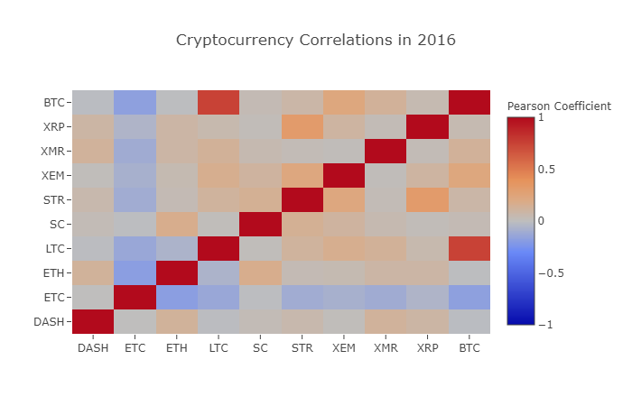
Here, the dark red value represents strong correlation (each currency is obviously highly correlated with itself), and the dark blue value represents inverse correlation. All colors in the middle - light blue/orange/grey/tawny - have values that represent varying degrees of weak correlation or non-correlation.
What does this chart tell us? Fundamentally, it shows the fluctuation of different digital currency prices in 2016, with little statistically significant correlation.
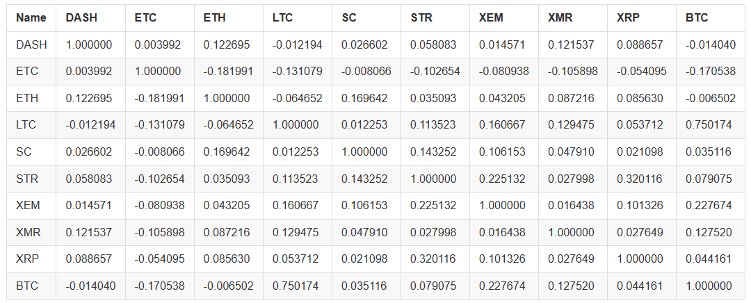
Now, in order to verify our hypothesis that "the correlation of digital currency has increased in recent months", we will use the data from 2017 to repeat the same test.
            javascript

            combined_df_2017 = combined_df[combined_df.index.year == 2017]
combined_df_2017.pct_change().corr(method='pearson')
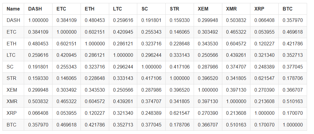
Are the data above more relevant? Are they sufficient to be used as a judgment standard for investment? The answer is no.
However, it is worth noting that almost all digital currencies have become increasingly interconnected.
            javascript

            correlation_heatmap(combined_df_2017.pct_change(), "Cryptocurrency Correlations in 2017")
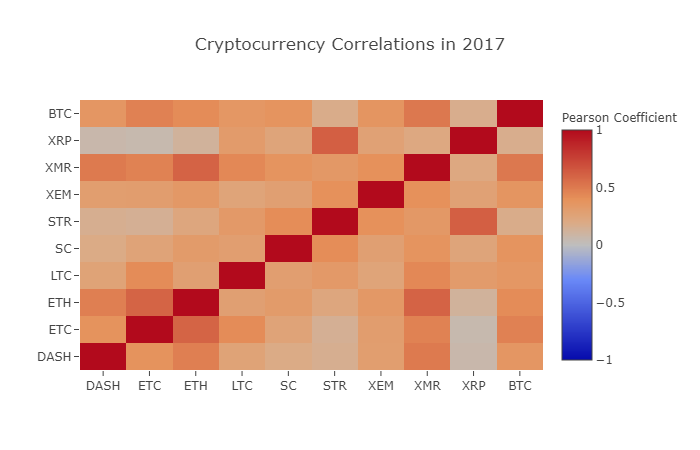
As we can see from the chart above, things are becoming more and more interesting.
Why does this happen?
Good question! But the truth is, I'm not sure...
My first reaction is that hedge funds have recently started trading publicly in the digital currency market. These funds hold much more capital than ordinary traders. When a fund hedges its invested capital among multiple digital currencies, it uses similar trading strategies for each currency according to independent variables (such as the stock market). From this perspective, it makes sense that this trend of increasing correlation would occur.
A deeper understanding of XRP and STR
For example, it is obvious from the chart above that XRP (Ripple's token) has the least correlation with other digital currencies. However, one notable exception is STR (Stellar's token, officially known as "Lumens"), which has a strong correlation with XRP (correlation coefficient: 0.62).
Interestingly, Stellar and Ripple are very similar financial technology platforms, both of which aim to reduce the tedious steps of cross-border transfer between banks. It is conceivable that some big players and hedge funds may use similar trading strategies for their investments in Stellar and Ripple, considering the similarity of tokens used by blockchain services. This may be why XRP is more relevant to STR than other digital currencies.
Well, it's your turn!
The above explanations are largely speculative, and you may do better. Based on the foundation we have laid, you have hundreds of different ways to continue to explore the stories contained in the data.
The following are some of my suggestions. Readers can refer to the research in these directions:
- Add more digital currency data to the entire analysis.
- Adjust the time range and granularity of correlation analysis to obtain an optimized or coarse-grained trend view.
- Find trends from trading quantity or blockchain data mining. Compared with the original price data, if you want to predict future price fluctuations, you may need buy/sell quantity ratio data more.
- Add price data to stocks, commodities and fiat currencies to determine which of them is relevant to digital currencies (but don't forget the old saying "correlation does not imply causation").
- Use Event Registry, GDELT, and Google Trends to quantify the number of "hot words" surrounding a specific digital currency.
- Use the data to train a predictive machine learning model to predict tomorrow's prices. If you are more ambitious, you can even consider using recurrent neural network (RNN) for the above training.
- Use your analysis to create an automatic trading robot, which can be applied to the exchange website of "Poloniex" or "Coinbase" through the corresponding application programming interface (API). Please be careful: a robot with poor performance can easily destroy your assets instantly. The FMZ Quant platform (FMZ.COM) is recommended here.
The best part about Bitcoin and digital currency in general is their decentralized nature, which makes it more free and democratic than any other asset. You can share your analysis open-source, participate in the community, or write a blog! I hope you have mastered the skills required for self analysis and the ability to think dialectically when reading any speculative digital currency articles in the future, especially those predictions without data support. Thank you for reading. If you have any comments, suggestions or criticisms about this tutorial, please leave a message on https://www.fmz.com/bbs.
- 1