Achieving long-short positions balanced equity strategies with an orderly alignment

Achieving long-short positions balanced equity strategies with an orderly alignment

In the previous article (https://www.fmz.com/bbs-topic/9862), we introduced pair trading strategies and demonstrated how to create and automate trading strategies by using data and mathematical analysis.

The long-short positions balanced equity strategy is a natural extension of the pair trading strategy applicable to a basket of trading objects. It is particularly suitable for trading markets with many varieties and interrelationships, such as digital currency markets and commodity futures markets.

Basic principles

The long-short positions balanced equity strategy is to go long and go short a basket of trading targets simultaneously. Just like pair trading, it determines which investment target is cheap and which investment target is expensive. The difference is that the long-short positions balanced equity strategy will arrange all investment targets in a stock selection pool to determine which investment targets are relatively cheap or expensive. Then, it will go long the top n investment targets based on the ranking, and go short the bottom n investment targets in the same amount (total value of long positions = total value of short positions).

Do you remember what we said that pair trading is a market neutral strategy? The same is true for the long-short positions balanced equity strategy, because the equal amount of long and short positions ensures that the strategy will remain market neutral (not affected by market fluctuations). The strategy is also statistically robust; By ranking the investment targets and holding long positions, you can open positions on your ranking model many times, not just one time risk opening position. You are purely betting on the quality of your ranking scheme.

What is the ranking scheme?

The ranking scheme is a model that can assign priority to each investment subject according to the expected performance. The factors can be value factors, technical indicators, pricing models or a combination of all the above factors. For example, you can use momentum indicators to rank a series of trend tracking investment targets: it is expected that the investment targets with the highest momentum will continue to perform well and get the highest ranking; The investment object with the least momentum has the worst performance and the lowest returns.

The success of this strategy almost entirely depends on the ranking scheme used, that is, your ranking scheme can separate the high performance investment target from the low performance investment target, so as to better realize the return of the strategy of long and short positions investment targets. Therefore, it is very important to develop a ranking scheme.

How to make a ranking scheme?

Once we have determined the ranking scheme, we do hope to make a profit from it. We do this by investing the same amount of capital to go long the top investment targets and go short the bottom investment targets. This ensures that the strategy will only make profits in proportion to the quality of the ranking, and it will be “market neutral”.

Suppose you are ranking all investment targets m, and you have n dollars for investment, and you want to hold a total of 2p (where m>2p) positions. If the investment object ranking rank 1 is expected to perform the worst, the investment object ranking m is expected to perform the best:

• You rank the investment objects as: 1,…,p position, go short the investment target of 2/2p USD.

• You rank the investment objects as: m-p,…,m position, go long the investment target of n/2p USD.

Note: Because the price of investment subject matter caused by price fluctuation will not always divide n/2p evenly, and some investment subject matters must be purchased with integers, there will be some inaccurate algorithms, which should be as close to this number as possible. For strategies running n=100000 and p=500, we see that:

n/2p = 100000/1000 = 100

This will cause a big problem for scores with a price greater than 100 (such as the commodity futures market), because you cannot open a position with a fractional price (this problem does not exist in digital currency markets). We mitigate this situation by reducing fractional price transactions or increasing capital.

Let’s take a hypothetical example.

• Build our research environment on the FMZ Quant platform

First of all, in order to work smoothly, we need to build our research environment. In this article, we use the FMZ Quant platform (FMZ.COM) to build our research environment, mainly to use the convenient and fast API interface and the well-packaged Docker system of this platform later.

In the official name of the FMZ Quant platform, this Docker system is called the Docker system.

Please refer to my previous article on how to deploy a docker and robot: https://www.fmz.com/bbs-topic/9864.

Readers who want to purchase their own cloud computing server to deploy dockers can refer to this article: https://www.fmz.com/digest-topic/5711.

After deploying the cloud computing server and the docker system successfully, next, we will install the present largest artifact of Python: Anaconda

In order to realize all the relevant program environments (dependency libraries, version management, etc.) required in this article, the simplest way is to use Anaconda. It is a packaged Python data science ecosystem and dependency library manager.

For the installation method of Anaconda, please refer to the official guide of Anaconda: https://www.anaconda.com/distribution/.

This article will also use numpy and pandas, two popular and important libraries in Python scientific computing.

The above basic work can also refer to my previous articles, which introduce how to set up the Anaconda environment and the numpy and pandas libraries. For details, please refer to: https://www.fmz.com/digest-topic/9863.

We generate random investment targets and random factors to rank them. Let’s assume that our future returns actually depend on these factor values.

import numpy as np
import statsmodels.api as sm
import scipy.stats as stats
import scipy
import matplotlib.pyplot as plt
import seaborn as sns
import pandas as pd
## PROBLEM SETUP ##
# Generate stocks and a random factor value for them
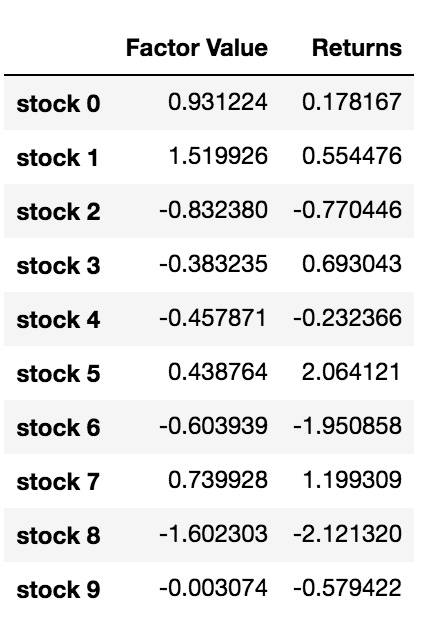
stock_names = ['stock ' + str(x) for x in range(10000)]
current_factor_values = np.random.normal(0, 1, 10000)
# Generate future returns for these are dependent on our factor values
future_returns = current_factor_values + np.random.normal(0, 1, 10000)
# Put both the factor values and returns into one dataframe
data = pd.DataFrame(index = stock_names, columns=['Factor Value','Returns'])
data['Factor Value'] = current_factor_values
data['Returns'] = future_returns
# Take a look
data.head(10)

Now that we have the factor values and returns, we can see what happens if we rank the investment targets based on the factor values and then open long and short positions.

# Rank stocks
ranked_data = data.sort_values('Factor Value')
# Compute the returns of each basket with a basket size 500, so total (10000/500) baskets
number_of_baskets = int(10000/500)
basket_returns = np.zeros(number_of_baskets)
for i in range(number_of_baskets):
    start = i * 500
    end = i * 500 + 500 
    basket_returns[i] = ranked_data[start:end]['Returns'].mean()
# Plot the returns of each basket
plt.figure(figsize=(15,7))
plt.bar(range(number_of_baskets), basket_returns)
plt.ylabel('Returns')
plt.xlabel('Basket')
plt.legend(['Returns of Each Basket'])
plt.show()

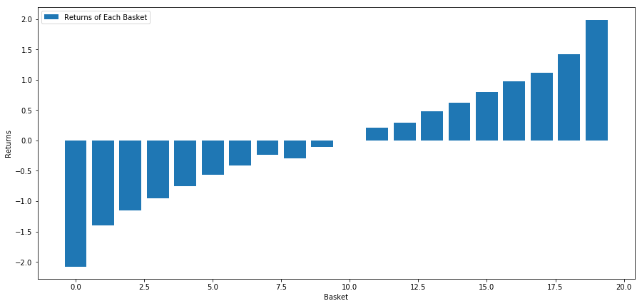
Our strategy is to go long the first ranked basket of investment target pools; go short of the tenth ranked basket. The returns for this strategy are:

basket_returns[number_of_baskets-1] - basket_returns[0]

The result is: 4.172

Put money on our ranking model so that it can separate high-performance investment targets from low-performance investment targets.

In the rest of this article, we will discuss how to evaluate the ranking scheme. The advantage of ranking-based arbitrage is that it is not affected by market disorder, instead the market disorder can be used.

Let’s consider a-real world example.

We loaded data for 32 stocks in different industries in the S&P 500 index and tried to rank them.

from backtester.dataSource.yahoo_data_source import YahooStockDataSource
from datetime import datetime
startDateStr = '2010/01/01'
endDateStr = '2017/12/31'
cachedFolderName = '/Users/chandinijain/Auquan/yahooData/'
dataSetId = 'testLongShortTrading'
instrumentIds = ['ABT','AKS','AMGN','AMD','AXP','BK','BSX',
                'CMCSA','CVS','DIS','EA','EOG','GLW','HAL',
                'HD','LOW','KO','LLY','MCD','MET','NEM',
                'PEP','PG','M','SWN','T','TGT',
                'TWX','TXN','USB','VZ','WFC']
ds = YahooStockDataSource(cachedFolderName=cachedFolderName,
                            dataSetId=dataSetId,
                            instrumentIds=instrumentIds,
                            startDateStr=startDateStr,
                            endDateStr=endDateStr,
                            event='history')
price = 'adjClose'

Let’s use the standardized momentum indicator for a one-month time period as the basis for ranking.

## Define normalized momentum
def momentum(dataDf, period):
    return dataDf.sub(dataDf.shift(period), fill_value=0) / dataDf.iloc[-1]
## Load relevant prices in a dataframe
data = ds.getBookDataByFeature()['Adj Close']
#Let's load momentum score and returns into separate dataframes
index = data.index
mscores = pd.DataFrame(index=index,columns=assetList)
mscores = momentum(data, 30)
returns = pd.DataFrame(index=index,columns=assetList)
day = 30

Now we will analyze the behavior of our stock and see how our stock operates in the market in the ranking factor we choose.

Analyze the data

Stock behavior

Let’s see how our selected basket of stocks performs in our ranking model. To do this, let’s calculate the weekly forward return for all stocks. Then we can see the correlation between the 1-week forward return of each stock and the momentum of the previous 30 days. The stocks showing positive correlation are trend followers, while the stocks showing negative correlation are mean reversals.

# Calculate Forward returns
forward_return_day = 5
returns = data.shift(-forward_return_day)/data -1
returns.dropna(inplace = True)
# Calculate correlations between momentum and returns
correlations = pd.DataFrame(index = returns.columns, columns = ['Scores', 'pvalues'])
mscores = mscores[mscores.index.isin(returns.index)]
for i in correlations.index:
    score, pvalue = stats.spearmanr(mscores[i], returns[i])
    correlations[‘pvalues’].loc[i] = pvalue
    correlations[‘Scores’].loc[i] = score
correlations.dropna(inplace = True)
correlations.sort_values('Scores', inplace=True)
l = correlations.index.size
plt.figure(figsize=(15,7))
plt.bar(range(1,1+l),correlations['Scores'])
plt.xlabel('Stocks')
plt.xlim((1, l+1))
plt.xticks(range(1,1+l), correlations.index)
plt.legend(['Correlation over All Data'])
plt.ylabel('Correlation between %s day Momentum Scores and %s-day forward returns by Stock'%(day,forward_return_day));
plt.show()

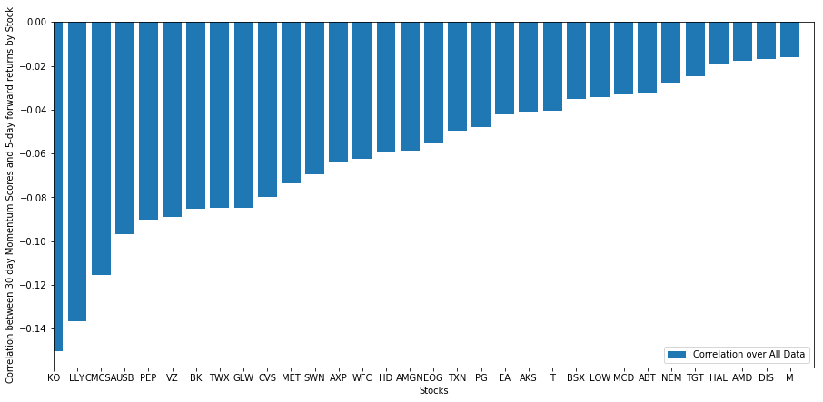
All our stocks have a mean reversion to a certain extent! (Obviously, the universe we chose works like this.) This tells us that if stocks rank top in momentum analysis, we should expect them to perform poorly next week.

Correlation between ranking of momentum analysis scores and returns

Next, we need to see the correlation between our ranking scores and the overall forward returns of the market, that is, the relationship between the predicted return rate and our ranking factor. Can a higher correlation level predict a lower relative return, or vice versa?

For this purpose, we calculate the daily correlation between the 30-day momentum of all stocks and the 1-week forward return.

correl_scores = pd.DataFrame(index = returns.index.intersection(mscores.index), columns = ['Scores', 'pvalues'])
for i in correl_scores.index:
    score, pvalue = stats.spearmanr(mscores.loc[i], returns.loc[i])
    correl_scores['pvalues'].loc[i] = pvalue
    correl_scores['Scores'].loc[i] = score
correl_scores.dropna(inplace = True)
l = correl_scores.index.size
plt.figure(figsize=(15,7))
plt.bar(range(1,1+l),correl_scores['Scores'])
plt.hlines(np.mean(correl_scores['Scores']), 1,l+1, colors='r', linestyles='dashed')
plt.xlabel('Day')
plt.xlim((1, l+1))
plt.legend(['Mean Correlation over All Data', 'Daily Rank Correlation'])
plt.ylabel('Rank correlation between %s day Momentum Scores and %s-day forward returns'%(day,forward_return_day));
plt.show()

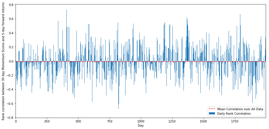
The daily correlations show a very complex but very slight correlation (which is expected since we said all stocks will return to the mean). We also have to look at the average monthly correlation of the forward return of 1 month.

monthly_mean_correl =correl_scores['Scores'].astype(float).resample('M').mean()
plt.figure(figsize=(15,7))
plt.bar(range(1,len(monthly_mean_correl)+1), monthly_mean_correl)
plt.hlines(np.mean(monthly_mean_correl), 1,len(monthly_mean_correl)+1, colors='r', linestyles='dashed')
plt.xlabel('Month')
plt.xlim((1, len(monthly_mean_correl)+1))
plt.legend(['Mean Correlation over All Data', 'Monthly Rank Correlation'])
plt.ylabel('Rank correlation between %s day Momentum Scores and %s-day forward returns'%(day,forward_return_day));
plt.show()

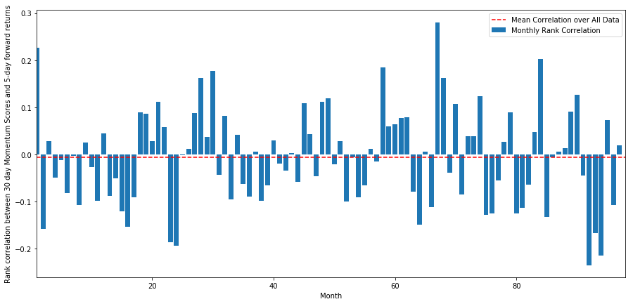
We can see that the average correlation is slightly negative again, but it also changes greatly every month.

Average return on a basket of stocks

We have calculated the return on a basket of stocks taken from our ranking. If we rank all the stocks and divide them into nn groups, what is the average return of each group?

The first step is to create a function that will give the average return and ranking factor of each basket given each month.

def compute_basket_returns(factor, forward_returns, number_of_baskets, index):
data = pd.concat([factor.loc[index],forward_returns.loc[index]], axis=1)
    # Rank the equities on the factor values
    data.columns = ['Factor Value', 'Forward Returns']
    data.sort_values('Factor Value', inplace=True)
    # How many equities per basket
    equities_per_basket = np.floor(len(data.index) / number_of_baskets)
basket_returns = np.zeros(number_of_baskets)
# Compute the returns of each basket
    for i in range(number_of_baskets):
        start = i * equities_per_basket
        if i == number_of_baskets - 1:
            # Handle having a few extra in the last basket when our number of equities doesn't divide well
            end = len(data.index) - 1
        else:
            end = i * equities_per_basket + equities_per_basket
        # Actually compute the mean returns for each basket
        #s = data.index.iloc[start]
        #e = data.index.iloc[end]
        basket_returns[i] = data.iloc[int(start):int(end)]['Forward Returns'].mean()
        
    return basket_returns

When we rank stocks based on this score, we calculate the average return of each basket. This should allow us to understand their relationship for a long time.

number_of_baskets = 8
mean_basket_returns = np.zeros(number_of_baskets)
resampled_scores = mscores.astype(float).resample('2D').last()
resampled_prices = data.astype(float).resample('2D').last()
resampled_scores.dropna(inplace=True)
resampled_prices.dropna(inplace=True)
forward_returns = resampled_prices.shift(-1)/resampled_prices -1
forward_returns.dropna(inplace = True)
for m in forward_returns.index.intersection(resampled_scores.index):
    basket_returns = compute_basket_returns(resampled_scores, forward_returns, number_of_baskets, m)
    mean_basket_returns += basket_returns
mean_basket_returns /= l    
print(mean_basket_returns)
# Plot the returns of each basket
plt.figure(figsize=(15,7))
plt.bar(range(number_of_baskets), mean_basket_returns)
plt.ylabel('Returns')
plt.xlabel('Basket')
plt.legend(['Returns of Each Basket'])
plt.show()

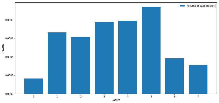
It seems that we can separate high performers from low performers.

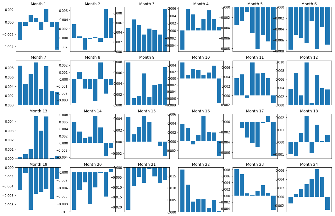
Margin (basis) consistency

Of course, these are just average relationships. In order to understand how consistent the relationship is and whether we are willing to trade, we should change our approach and attitude to it over time. Next, we will look at their monthly interest margin (basis) for the previous two years. We can see more changes and conduct further analysis to determine whether this momentum score can be traded.

total_months = mscores.resample('M').last().index
months_to_plot = 24
monthly_index = total_months[:months_to_plot+1]
mean_basket_returns = np.zeros(number_of_baskets)
strategy_returns = pd.Series(index = monthly_index)
f, axarr = plt.subplots(1+int(monthly_index.size/6), 6,figsize=(18, 15))
for month in range(1, monthly_index.size):
    temp_returns = forward_returns.loc[monthly_index[month-1]:monthly_index[month]]
    temp_scores = resampled_scores.loc[monthly_index[month-1]:monthly_index[month]]
    for m in temp_returns.index.intersection(temp_scores.index):
        basket_returns = compute_basket_returns(temp_scores, temp_returns, number_of_baskets, m)
        mean_basket_returns += basket_returns
    
    strategy_returns[monthly_index[month-1]] = mean_basket_returns[ number_of_baskets-1] - mean_basket_returns[0]
    
    mean_basket_returns /= temp_returns.index.intersection(temp_scores.index).size
    
    r = int(np.floor((month-1) / 6))
    c = (month-1) % 6
    axarr[r, c].bar(range(number_of_baskets), mean_basket_returns)
    axarr[r, c].xaxis.set_visible(False)
    axarr[r, c].set_title('Month ' + str(month))
plt.show()

plt.figure(figsize=(15,7))
plt.plot(strategy_returns)
plt.ylabel('Returns')
plt.xlabel('Month')
plt.plot(strategy_returns.cumsum())
plt.legend(['Monthly Strategy Returns', 'Cumulative Strategy Returns'])
plt.show()

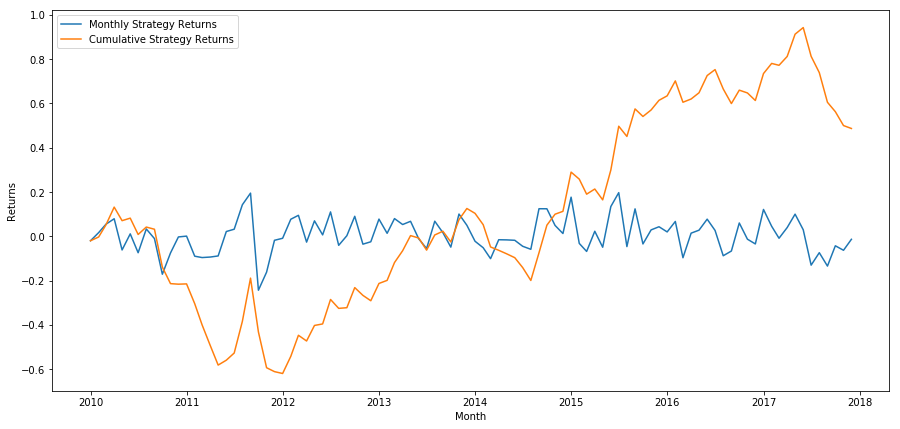
Finally, if we go long the last basket and go short the first basket every month, then let’s look at the returns (assuming equal capital allocation per security).

total_return = strategy_returns.sum()
ann_return = 100*((1 + total_return)**(12.0 /float(strategy_returns.index.size))-1)
print('Annual Returns: %.2f%%'%ann_return)

Annual return rates: 5.03%

We can see that we have a very weak ranking scheme, which can only gently distinguish high performance stocks from low performance stocks. In addition, this ranking scheme is not consistent and varies greatly every month.

Find the right ranking scheme

In order to realize the long-short balanced equity strategy, actually, you only need to determine the ranking scheme. Everything after that is mechanical. Once you have a long-short balanced equity strategy, you can exchange different ranking factors without much change. It’s a very convenient way to iterate your ideas quickly without worrying about adjusting all the code each time.

The ranking scheme can also come from almost any model. It is not necessarily a value-based factor model. It can be a machine learning technology that can predict returns one month in advance and rank according to this level.

Selection and evaluation of ranking scheme

Ranking scheme is the advantage and the most important part of the long-short balanced equity strategy. Choosing a good ranking scheme is a systematic project, and there is no easy answer.

A good starting point is to select existing known technologies and see if you can modify them slightly to get higher returns. Here we will discuss several starting points:

• Clone and adjustment: Choose a topic that is often discussed, and see if you can modify it slightly to gain advantages. Generally, the publicly available factors will no longer have trading signals, because they have completely arbitraged out of the market. But sometimes they will lead you in the right direction.

• Pricing model: Any model that predicts future returns may be a factor that can potentially be used to rank your basket of trading objects. You can take any complex pricing model and convert it into a ranking scheme.

• Price-based factors (technical indicators): price-based factors, as discussed today, obtain information about the historical price of each equity and use it to generate factor values. Examples might be moving average indicators, momentum indicators, or volatility indicators.

• Regression and momentum: It is worth noting that some factors believe that once prices move in one direction, they will continue to do so, while some factors are just the opposite. Both are effective models for different time horizons and assets, and it is important to study whether the basic behavior is based on momentum or regression.

• Basic factor (value-based): This is a combination of basic values, such as PE, dividends, etc. The basic value contains information related to the real world facts of the company, so it can be more powerful than the price in many aspects.

Ultimately, the development predictor is an arms race, and you are trying to stay one step ahead. Factors will be arbitrage from the market and have a useful life, so you must constantly work to determine how many recessions your factors have experienced and what new factors can be used to replace them.

Other considerations

• Rebalance frequency

Each ranking system predicts returns in a slightly different time frame. The mean regression based on price may be predictable in a few days, while the factor model based on value may be predictive in a few months. It is important to determine the time range that the model should predict, and perform statistical verification before executing the strategy. Of course, you don’t want to overfit by trying to optimize the rebalance frequency. You will inevitably find a random frequency that is better than other frequencies. Once you have determined the time range of the ranking scheme prediction, try to rebalance at about this frequency to make full use of your model.

• Capital capacity and transaction costs

Each strategy has the minimum and maximum capital volume, and the minimum threshold is usually determined by the transaction cost.

Trading too many stocks will lead to high transaction costs. If you want to buy 1,000 shares, it will cost thousands of dollars on each rebalancing. Your capital base must be high enough so that transaction costs can account for a small part of the returns your strategy generates. For example, if your capital is $100,000 and your strategy earns 1% ($1,000) per month, all these returns will be consumed by transaction costs. You need to run the strategy with millions of dollars of capital to earn more than 1,000 shares.

The lowest asset threshold mainly depends on the number of shares traded. However, the maximum capacity is also very high. The long-short balanced equity strategy can trade hundreds of millions of dollars without losing the advantage. This is a fact, because this strategy is relatively infrequent to rebalance. The dollar value of each share will be very low when the total assets are divided by the number of stocks traded. You don’t have to worry about whether your trading volume will affect the market. Suppose you trade 1,000 shares, that is, 100,000,000 dollars. If you rebalance the entire portfolio every month, each stock will only trade $100,000 a month, which is not enough to be an important market share for most securities.

Related

More