

Neural Networks and Digital Currency Quantitative Trading Series (1) - LSTM Predicts Bitcoin Price
1. Brief introduction
The deep neural network has become more and more popular in recent years. It has solved the problems that could not be solved in the past in many fields and has demonstrated its strong ability. In the prediction of time series, the commonly used neural network price is RNN, because it has not only current data input, but also historical data input. Of course, when we talk about RNN price prediction, we often talk about one of the RNNs: LSTM. This paper will build a model to predict the price of Bitcoin based on PyTorch. Although there is a lot of relevant information on the Internet, it is still not thorough enough, and there are relatively few people who use PyTorch. It is still necessary to write an article. The final result is to use the opening price, closing price, highest price, lowest price, and trading volume of Bitcoin to predict the next closing price. My personal knowledge of neural networks is limited, and I hope for your criticism and corrections.
This tutorial is produced by the FMZ Quant Trading platform (www.fmz.com). Welcome to join the QQ group: 863946592 for communication.
2. Data and reference
Bitcoin price data sourced from FMZ Quant Trading platform: https://www.quantinfo.com/Tools/View/4.html.
A related example of price prediction: https://yq.aliyun.com/articles/538484.
A detailed introduction to the RNN model: https://zhuanlan.zhihu.com/p/27485750.
Understanding the input and output of RNN: https://www.zhihu.com/question/41949741/answer/318771336.
About pytorch: the official documentation: https://pytorch.org/docs, For other information, you can search by yourself.
In addition, you need some prior knowledge to read this article, such as pandas/python/data processing, but it doesn't matter if you don't.
3. Parameters of the pytorch LSTM model
Parameters of LSTM:
The first time I saw these dense parameters on the document, my reaction was: What the hell is this?
As I read slowly, I finally understood.
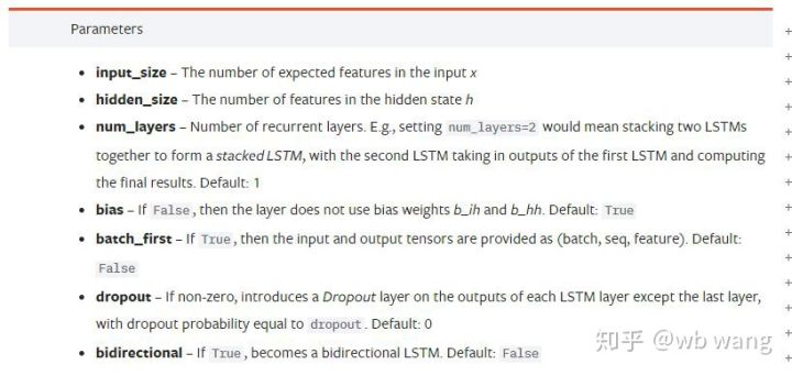
input_size: Input the characteristic size of vector x. If the closing price is predicted by the closing price, then input_size=1; If the closing price is predicted by high opening and low closing, then input_size=4.
hidden_size: Implicit layer size
num_layers: Number of layers of RNN.
batch_first: If true, the first input dimension is batch_size, which is also very confusing, and it will be described in detail below.
Enter the data parameters:
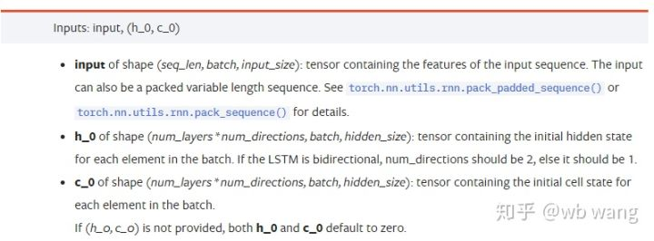
input: The specific input data is a three-dimensional tensor, and the specific shape is: (seq_len, batch, input_size). Where, seq_len refers to the length of the sequence, that is, how long the LSTM needs to consider the historical data. Note that this refers to the format of the data only, not the internal structure of the LSTM. The same LSTM model can enter different seqs_len's data, which can give prediction results; batch refers to the size of the batch, representing how many different groups of data; input_size is the previous input_size.
h_0: Initial hidden state, shape as (num_layers * num_directions, batch, hidden_size), if it is a two-way network, num_directions=2.
c_0: Initial cell state, shape as above, can be unspecified.
Output parameters:
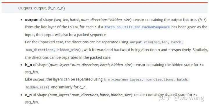
output: The shape of the output (seq_len, batch, num_directions * hidden_size), note that it is related to the model parameter batch_first.
h_n: The h state at the moment of t = seq_len, same shape as h_0.
c_n: The c state at the moment of t = seq_len, same shape as c_0.
4. A simple example of LSTM input and output
Import the required package first
import pandas as pd
import numpy as np
import torch
import torch.nn as nn
import matplotlib.pyplot as plt
Define the LSTM model
LSTM = nn.LSTM(input_size=5, hidden_size=10, num_layers=2, batch_first=True)
Prepare the input data
            x = torch.randn(3,4,5)
# The value of x is:
tensor([[[ 0.4657,  1.4398, -0.3479,  0.2685,  1.6903],
         [ 1.0738,  0.6283, -1.3682, -0.1002, -1.7200],
         [ 0.2836,  0.3013, -0.3373, -0.3271,  0.0375],
         [-0.8852,  1.8098, -1.7099, -0.5992, -0.1143]],

        [[ 0.6970,  0.6124, -0.1679,  0.8537, -0.1116],
         [ 0.1997, -0.1041, -0.4871,  0.8724,  1.2750],
         [ 1.9647, -0.3489,  0.7340,  1.3713,  0.3762],
         [ 0.4603, -1.6203, -0.6294, -0.1459, -0.0317]],

        [[-0.5309,  0.1540, -0.4613, -0.6425, -0.1957],
         [-1.9796, -0.1186, -0.2930, -0.2619, -0.4039],
         [-0.4453,  0.1987, -1.0775,  1.3212,  1.3577],
         [-0.5488,  0.6669, -0.2151,  0.9337, -1.1805]]])
The shape of x is (3,4,5), because we defined batch_first=True previously, the size of batch_size at this time is 3, sqe_len is 4, input_size is 5. X [0] represents the first batch.
If batch_first is not defined, the default value is False, then the data representation is completely different at this time. The batch size is 4, sqe_len is 3, input_size is 5. At this time, x [0] represents the data of all batches when t=0, and so on. I feel that this setting is not intuitive, so I added the parameter batch_first=True.
The data conversion between the two is also very convenient: x.permute (1,0,2)
Input and output
The shape of input and output of LSTM is very confusing, and the following figure can help us understand:
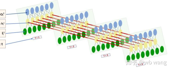
From: https://www.zhihu.com/question/41949741/answer/318771336.
            x = torch.randn(3,4,5)
h0 = torch.randn(2, 3, 10)
c0 = torch.randn(2, 3, 10)
output, (hn, cn) = LSTM(x, (h0, c0))
print(output.size()) # Thinking about it, what would be the size of the output if batch_first=False?
print(hn.size())
print(cn.size())
# result
torch.Size([3, 4, 10])
torch.Size([2, 3, 10])
torch.Size([2, 3, 10])
Observe the output result, which is consistent with the previous parameter interpretation. Note that the second value of hn.size() is 3, which is consistent with the size of batch_size, which means that the intermediate state is not saved in hn, only the last step is saved.
Since our LSTM network has two layers, in fact, the output of the last layer of hn is the value of output. The shape of output is [3, 4, 10], which saves the results at all times of t=0,1,2,3, so:
            hn[-1][0] == output[0][-1] # The output of the first batch at the last level of hn is equal to the output of the first batch at t=3.
hn[-1][1] == output[1][-1]
hn[-1][2] == output[2][-1]
5. Prepare Bitcoin market data
So much has been said before, which is just a prelude. It is very important to understand the input and output of LSTM. Otherwise, it is easy to make mistakes by randomly extracting some codes from the Internet. Because of the strong ability of LSTM in time series, even if the model is wrong, good results can be obtained in the end.
Data acquisition
The market data of BTC_USD trading pair in Bitfinex Exchange is used.
import requests
import json
resp = requests.get('https://www.quantinfo.com/API/m/chart/history?symbol=BTC_USD_BITFINEX&resolution=60&from=1525622626&to=1562658565')
data = resp.json()
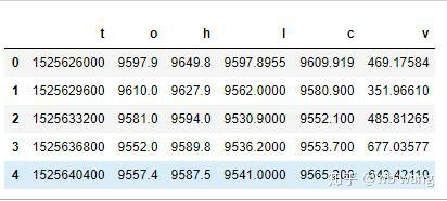
df = pd.DataFrame(data,columns = ['t','o','h','l','c','v'])
print(df.head(5))
The data format is as follows:
Data pre-processing
            df.index = df['t'] # index is set to timestamp
df = (df-df.mean())/df.std() # The standardization of the data, otherwise the loss of the model will be very large, which is not conducive to convergence.
df['n'] = df['c'].shift(-1) # n is the closing price of the next period, which is our forecast target.
df = df.dropna()
df = df.astype(np.float32) # Change the data format to fit pytorch.
The method of data standardization is very rough, and there will be some problems. Just for demonstration, you can use data standardization such as return rates.
Prepare training data
            seq_len = 10 # Input 10 periods of data
train_size = 800 # Training set batch_size
def create_dataset(data, seq_len):
    dataX, dataY=[], []
    for i in range(0,len(data)-seq_len, seq_len):
        dataX.append(data[['o','h','l','c','v']][i:i+seq_len].values)
        dataY.append(data['n'][i:i+seq_len].values)
    return np.array(dataX), np.array(dataY)
data_X, data_Y = create_dataset(df, seq_len)
train_x = torch.from_numpy(data_X[:train_size].reshape(-1,seq_len,5)) # The change in shape, -1 represents the value that will be calculated automatically.
train_y = torch.from_numpy(data_Y[:train_size].reshape(-1,seq_len,1))
The final shapes of train_x and train_y are: torch.Size ([800, 10, 5]), torch.Size ([800, 10, 1]). Because our model predicts the closing price of the next period based on the data of 10 periods, there are 800 batches in theory, as long as there are 800 predicted closing prices. But train_y in each batch has 10 data. In fact, the intermediate result of each batch prediction is reserved. When calculating the final loss, all 10 prediction results can be taken into account and compared with the actual value in train_y. Theoretically, we can calculate the Loss of the last prediction result only. Because the LSTM model does not contain seq_len parameter actually, so the model can be applied to different lengths, and the prediction results in the middle are also meaningful, so I prefer to combine and calculate Loss.
Note that when preparing training data, the movement of the window is jumping, and the data already used is no longer used. Of course, the window can also be moved one by one, so that the training set obtained is much larger. However, I felt that the adjacent batch data was too repetitive, so I adopted the current method.
6. Construct the LSTM model
The final model is constructed as follows, containing a two-layer LSTM and a Linear layer.
            class LSTM(nn.Module):
    def __init__(self, input_size, hidden_size, output_size=1, num_layers=2):
        super(LSTM, self).__init__()
        self.rnn = nn.LSTM(input_size,hidden_size,num_layers,batch_first=True)
        self.reg = nn.Linear(hidden_size,output_size) # Linear layer, output the result of LSTM into a value.

    def forward(self, x):
        x, _ = self.rnn(x) # If you don't understand the change of data dimension in forward propagation, you can debug it separately.
        x = self.reg(x)
        return x

net = LSTM(5, 10) # input_size is 5, which represents the high opening and low closing and trading volume. The implicit layer is 10.
7. Start training the model
Finally we start training, the code is as follows:
criterion = nn.MSELoss() # A simple mean square error loss function is used.
optimizer = torch.optim.Adam(net.parameters(),lr=0.01) # Optimize function, lr is adjustable.
for epoch in range(600): # Because of the speed, there are more epochs here.
out = net(train_x) # Due to the small amount of data, the full amount of data is directly used for calculation.
loss = criterion(out, train_y)
optimizer.zero_grad()
loss.backward() # Reverse propagation losses
optimizer.step() # Update parameters
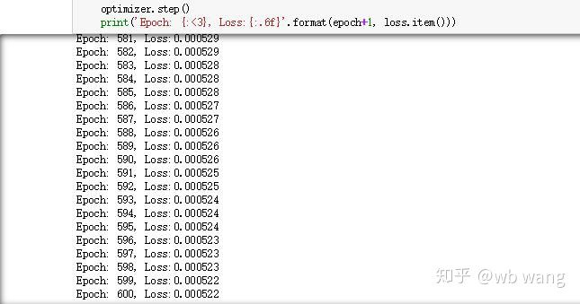
print('Epoch: {:<3}, Loss:{:.6f}'.format(epoch+1, loss.item()))
The training results are as follows:
8. Model Evaluation
The predicted value of the model:
            p = net(torch.from_numpy(data_X))[:,-1,0] # Only the last predicted value is taken here for comparison.
plt.figure(figsize=(12,8))
plt.plot(p.data.numpy(), label= 'predict')
plt.plot(data_Y[:,-1], label = 'real')
plt.legend()
plt.show()
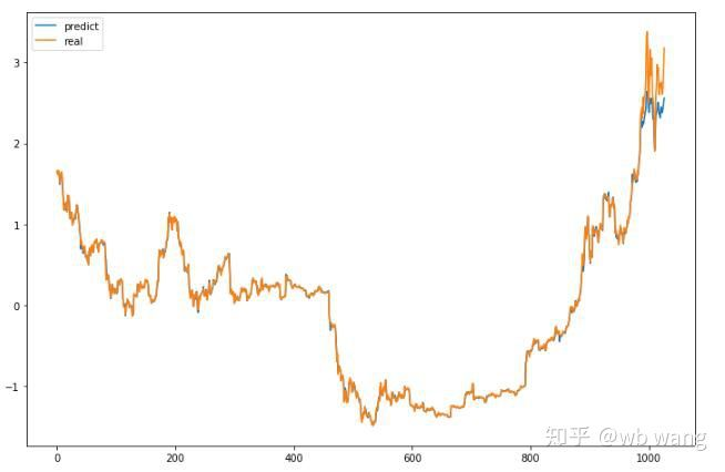
It can be seen from the chart that the training data (before 800) are very consistent, but the price of Bitcoin has risen in the later period. The model has not seen these data, so the prediction is inadequate. This also shows that there are problems in the standardization of data.
Although the predicted price may not be accurate, what is the accuracy of the prediction of the increasing and decreasing? Take a segment of forecast data to see:
            r = data_Y[:,-1][800:1000]
y = p.data.numpy()[800:1000]
r_change = np.array([1 if i > 0 else 0 for i in r[1:200] - r[:199]])
y_change = np.array([1 if i > 0 else 0 for i in y[1:200] - r[:199]])
print((r_change == y_change).sum()/float(len(r_change)))
As a result, the accuracy rate of forecasting the rise and fall reached 81.4%, which still exceeded my expectations. I don't know if there is something wrong.
Of course, this model is not applicable to the real bot, but it is simple and easy to understand. Just start with it. Next, there will be more introductory courses of neural network application in digital currency quantification.
- 1