Tycoon reveals algorithm trading: FMZ Quant platform market maker strategy

Digital currency algorithm transaction guide

In this article, we will discuss the design and implementation of the trading algorithm in Canadian currency. In particular, we focus on execution algorithms, market maker algorithms and several market microstructure considerations. We also studied the deviation of practice from theory, especially in dealing with the characteristics of the cryptocurrency market.

Execute algorithm

The goal of the execution algorithm is to transform the portfolio state into different states, while minimizing the cost of doing so. For example, if you want to increase the BTCUSD exposure rate by 1000, you may not want to enter the market orders into the BitMEX trading channel immediately, resulting in a large number of sliding points. On the contrary, you can consider getting the position you want slowly through the market and limit order combination of multiple different exchanges.

The execution algorithm usually has 3 layers: microtrader, microtrader and smart router.

The macrotrader layer splits large initial orders or parent orders into smaller orders that span time. Actually, it’s the scheduling part of the whole algorithm. VWAP, TWAP, and POV are common and simple examples of macrotrader algorithm. Generally, there are many different market impact models that can be used to design complex macrotrader layers. The design of market impact model focuses on the market’s response to execution. Will the market remain unchanged after implementation? Or go further? Or will it return to some extent? The two most groundbreaking market impact models are Almgren-Chriss (1999, 2000) permanent market impact model and Obizhueva-Wang (2013) transient market impact model. Based on this, in practice, the market impact is not permanent, so Obizhaeva-Wang seems to be more realistic, and since then, there have been many new models to solve its shortcomings.

Extended reading: the market influence begins to decay after the implementation of algorithmic trading: https://arxiv.org/pdf/1412.2152.pdf.

The microtrader layer determines whether to execute each sub-order as a market order or a limit order, and if it is a limit order, what price should be specified. There is little literature on microtrader design, because the size of sub-orders is usually a small part of the whole market, so how to implement it is not important. However, the digital currency market is different, because liquidity is very small, and even for sub-orders of ordinary size in practice, the sliding point is very obvious. The design of Microtrader usually focuses on time and depth, queue position and other characteristics of market microstructure. The market order (which is the same as the limit order if we ignore the delay) can be guaranteed to be executed, but the limit order has no such guarantee. If you cannot guarantee execution, you may fall behind the trading plan set by macrotrader.

The smart router layer decides how to direct orders to different exchanges. For example, if Kraken has 60% liquidity and GDAX (Coinbase ProPrime) has 40% liquidity at some specific price level, then microtrader should import orders to Kraken and GDAX exchanges at 60% and 40% respectively.

Now you can say that arbitrageurs and market makers in the market transfer liquidity from one exchange to another, so if you execute half of the orders in Kraken and wait for a few seconds, some liquidity will be supplemented from arbers and stat arbers to GDAX’s liquidity in Kraken, and you can complete the rest of the work at a similar price. However, even in this case, arbers will charge you extra fees for its own profits and transfer its hedging costs to Kraken’s market making fees. In addition, the number of orders issued by some market participants exceeds the scale they want to conduct on multiple exchanges, and the excess scale will be cancelled once the loss is stopped.

Finally, it is better to have your own local smart router. This local smart router also has the delay advantage for third-party smart router services. In the former case, you can route directly to the exchange, while in the latter case, you need to send a message to the third-party router service first, and then they send your order to the exchange (in addition, you must pay the router fee to the third party). The sum of any two legs of a triangle is greater than the third leg.

Market maker algorithm

Market making refers to providing immediate liquidity and compensation for other market participants. You take inventory risk in exchange for positive expected value. In the end, there are two reasons why market makers get compensation. First of all, market recipients have time preference and they need immediacy. In exchange, market makers who facilitate liquidity can compensate for their lower time preference and patience. Secondly, the PnL profit of market makers is left-leaning, and most traders usually have a right-leaning preference. In other words, market makers are similar to gambling companies in the gambling market, casinos, insurance companies and national lottery. They win small parts often, but they usually don’t lose great parts. As a compensation for the unexpected return profit, market makers are compensated for the expected value.

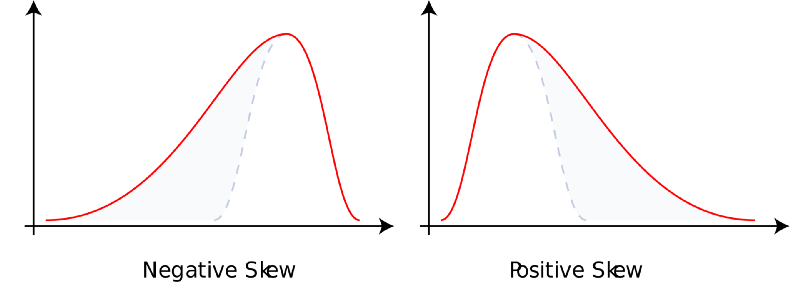
Extended reading: skewness: https://en.wikipedia.org/wiki/Skewness.

From a high-level perspective, limit orders are free options in other markets. The rest of the markets have the right but not the obligation to buy or sell assets at the limit price of the limit order. In a market where information is completely known, no one will sell free options. This is because the market as a whole is not a market with completely known information and it will never make sense to sell free options. On the other hand, if the market information is completely unknown, risk-neutral market makers are willing to sell these free limit order options with a small price difference, because all transactions are noise. Obviously, real market participants are mixed, and each participant has a unique degree of information known and unknown.

When designing the algorithm of market makers, there are three views to consider: market makers, market participants and other market makers.

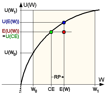
The market makers’ own views are represented by their inventories. If you already have too much asset risk, you may reduce your quotation, and vice versa. You do this for two different reasons. First of all, as a company, you have a certain degree of risk aversion (maybe less than individuals, but your currency utility curve is still concave).

The shape of this utility function has many structures (such as CARA, CRRA, and HARA, etc.). Secondly, as a passive liquidity provider in the market, you will face adverse selection risk. Positive liquidity recipients may know what you don’t have, or just be smarter than you. This is basically a matter of selling free options to the market.

In addition, even at the level of mechanical operation, the market order with market price order will also reduce the price in the way of pricing at market price, and the market order with higher quotation will be priced at market price. At the exact moment of any transaction, you are always on the wrong side. In addition, the quotation of market makers will have a passive market impact. In other words, the act of sending orders to the unfilled order book will keep the market away from you at least.

Extended reading: Risk aversion function: https://en.wikipedia.org/wiki/Risk_aversion.

The view of the market receiver is expressed by the order flow. The volume weighted frequency of order arrival as a function of depth should have some key attributes.

The function should be:

• 1. Decreasing,
• 2. Convex shape (it is difficult to explain with intuition, but it is clear in experience),
• 3. As the depth becomes infinite and asymptotically becomes zero, some formulas need this strength function to be differentiable for two consecutive times to be easy to deal with. This is a fine and reasonable assumption, but it is not necessary in the end. In addition, there are different formulas about how to calculate the “depth or distance from the top of the order book”. You can usually use some “reasonable middle price” or the best quotation of each corresponding trading party. There are different trade-offs between the two methods, and we will not discuss them here.

In addition, another unknown factor is how much the “fair intermediate price” should be. When sending and canceling deep orders, the middle price between the best buying price and the best selling price is vulnerable to noise price.

In addition, considering two cases with the same order book shape, the best bid of the latter order book will indicate that the fair price is lower than the best bid of the previous order book. Another question is whether the history of the order book is important. If so, should we pay close attention to the price time or the transaction volume time? So considering the characteristics of market flow, where should the best price limit order of market makers be placed? If you tighten the depth at the top of the order book, your depth orders will be many, but they are very few each time. If you tighten the depth at the bottom of the order book, your deep orders will be few, but there are many each time.

This is actually a convex optimization problem with a unique global maximum. Another factor to consider is that the order flow arrives across time, which looks like a “Poisson process”(https://zh.wikipedia.org/wiki/泊松过程). Some people think it is closer to the “Hawkes process”(http://jheusser.github.io/2013/09/08/hawkes.html). In addition, the buying and selling rebound that market makers try to capture is the shortest version of mean reversion. Because this ultra-short-term mean regression is scaled by local fluctuations, it is meaningful for market makers to expand their quotations when prices are high, and tighten their quotations when trading volume is low.

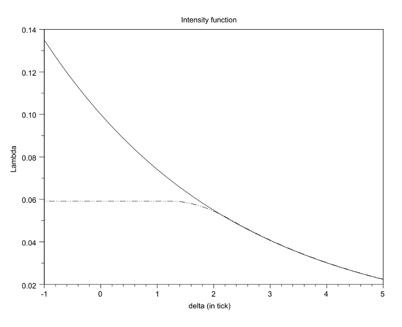
Extended reading: order arrival intensity with respect to depth (https://arxiv.org/pdf/1204.0148.pdf).

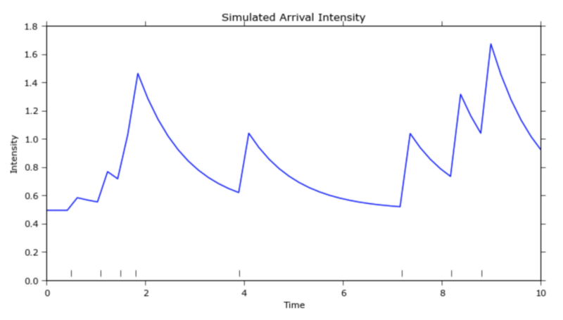
Extended reading: Hawkes Processes (http://jheusser.github.io/2013/09/08/hawkes.html)

The views of other market makers are represented by the order book, which reveals some information of other market makers. The buying price near the top of the order book is more than the selling price, indicating that other market makers are more willing to sell than buy. These market makers may already have a large amount of unbalanced inventory backlog, or they just think that prices are more likely to fall rather than rise in the short term. In either case, as a market maker, you can adjust the quotation according to the deviation of the chart order book.

In addition, you will often see this “penny price jump” behavior when market makers are competing with each other if the price jump is small. Market makers compete with each other for price until a surrender point is reached and only one “winner” gets the priority. After determining the winner, the runner-up usually falls back to the previous price jump next best bid or before the bid. If you lose the quotation priority, you may get a second quotation priority. This leads to a return phenomenon, that is, the winner now returns to a price adjustment and the same ladder in front of the runner-up, and the game of two climbers starts again.

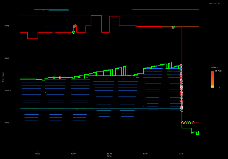
Extended reading: http://parasec.net/transmission/order-book-visualisation/

Finally, the signal of long-term orientation can cover the market making algorithm, where the goal of the market making algorithm is no longer to keep the inventory level or unchanged, but to consider some long-term goals and corresponding deviations to make it a reality.

Speed

Speed is important for two main reasons. First, you can close the order in the order book before canceling. Secondly, you can cancel the order in the order book before it is filled. In other words, you want to take the initiative in order filling and cancellation at all times. Arbitrage algorithms (active) and execution algorithms (active) care more about the former, while market making algorithms (passive) care more about the latter.

Generally, in principle, the strategies that benefit most from speed are those that have the simplest judgment logic. Any complex logic will inevitably slow down the round-trip time. These complex types of algorithmic strategies are Formula 1 racing cars in the trading world. Data validation, security checks, hardware settings, and layout methods may be deprived, all for the sake of speed. Skip OMS, EMS and PMS (Portfolio Management System) and connect the calculation logic on the GPU to the binary API interface of the same exchange directly. A fast and dangerous game.

Another type of speed-sensitive strategy, relative to the statistical arbitrage strategy, the server is actually located in multiple exchanges, rather than coexisting with a single exchange. Although they will not be the fastest data from any single exchange, they will obtain prices and they can take action on relevant and connection data before any other strategy.

Extended reading: The best intermediate trading node location of the world’s largest stock exchange (https://www.alexwg.org/publications/PhysRevE_82-056104.pdf)

In the speed game, the winner takes all. In the simplest example, if there is an arbitrage opportunity, anyone who can get the arbitrage opportunity first will gain profits. The second place gets crumbs, and the third place gets nothing. The income is likely to be distributed in the way of power law. (About power law: https://zh.wikipedia.org/wiki/冪定律)

The speed game is also a competition. Once everyone upgrades from optical fiber network to microwave or laser network, everyone will return to a fair competitive environment, and any initial advantage will be commercialized.

Size of price jump, preemption priority and queue position

Most engines that match orders follow the principle of price first, and then time first (proportional matching is a less common alternative, but we will not consider these now). The better price will be executed before the worse-price limit order is executed. For limited-price orders with the same price, the orders sent previously will be executed before the orders sent later.

Binance splits the order to up to 8 decimal places. If the price of the transaction is .000001, the price of .00000001 is 1% of the transaction. If the transaction price is .0001, the price of .00000001 is 1 bps (that is, one hop). This is a huge difference. In the former case, skipping a large order takes a complete point, so time priority is more important. In the latter case, it is 100 times cheaper, so price priority is more important.

In other words, if you have to pay 1% of the full amount to get the transaction priority, it may not be worth it, because you pay a relatively large amount, and increase the possibility of being closed by a relatively small amount, and it may be better to wait in line, but if you only need to pay 1 bps to get the transaction priority, you can do so, because you reduce the relatively small marginal cost, it increases the probability of a relatively large number of transactions at the same time. A smaller price jump is conducive to price priority, while a larger price jump is conducive to time priority.

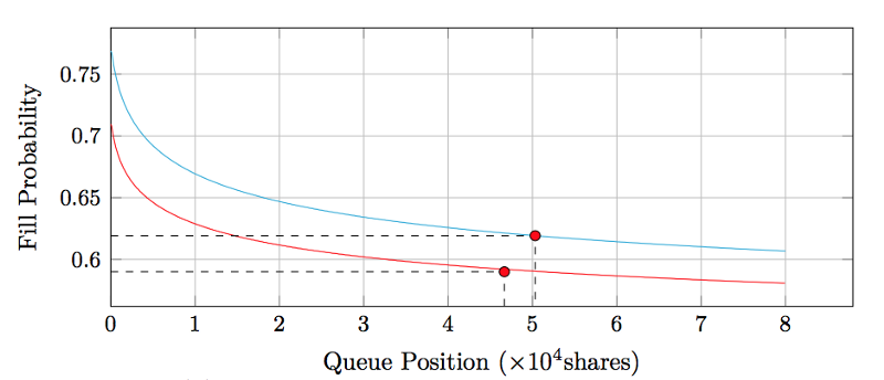
This naturally leads to the next question: What is the value of your queue position? (Extended reading: https://moallemi.com/ciamac/papers/queue-value-2016.pdf)

Order book Deltas

There are only two ways to reduce the number of transactions of orders in the order book: they are either cancelled voluntarily or closed. If the decrease is caused by the trading process, all other prices will also decrease due to the trading process. We can sort these transaction records by sorting them and mark whether each reduction is due to the transaction or the cancellation.

Intuitively, trading means that both parties agree to trade at a specific price, while cancellation means that one party decides not to buy or sell at a specific price. Therefore, on the surface, we may say that the cancellation with the best offer is a very strong signal that the market price will move downward in the short term, followed by a trade price right behind it.

On the other hand, the price in the order book starts to rise. There is only one possibility: increase the number of remaining limit orders.

The increment and decrement in the order book show the private will of market participants, thus providing a signal of short-term price movement.

Better price index and optimal transaction cost

At present, most price indexes obtain trading data from multiple exchanges and aggregate together them to obtain the volume-weighted average price. In particular, the Tradeblock index will also increase the penalty mechanism of the exchange weight, which is strongly correlated with inactivity and exchanges that deviate too far from the price. Besides, what else can we improve?

On GDAX, the maker fee is 0 basis points and the taker fee is 30 basis points. For example, the transaction price is shown as $4000/BTC, which is actually the seller’s selling price of $4000/BTC and the buyer’s buying price of $4012/BTC. The “reasonable price” of this transaction should be close to $4006/BTC rather than the actual displayed price. On the other hand, since Bittrex’s 25bps fee applies to both makers and takers, the actual price is the displayed price. In other words, the display price of $4000/BTC is actually that the buyer buys at $4010/BTC, and the seller sells at $3990/BTC. The average price is the display price itself.

Therefore, from the perspective of price discovery, the prices of transaction records are not directly comparable among exchanges, and should be standardized after the construction of the price index takes into account the above conditions. Of course, there are some complex factors that lead to different commissions based on the volume of transactions. For example, some exchanges set and charge the maker and maker fees according to the volume of transactions. This also implies two interesting inferences.

First of all, price discovery is limited. In some ways, it also strengthens the asymmetry between the exchanges about the maker and the maker costs. Assuming that most accounts of GDAX are at the level of 0/30 basis points of maker and taker fees and that GDAX usually has a penny difference in its BTCUSD order book, the price displayed in the bid for each transaction is about “fair value”, which is within 15 points higher than the spot and each transaction, and the displayed price between them is about “fair value”. Therefore, the “fair price” in the calm period oscillates rapidly between these two points, and the price discovery between them has not been further refined.

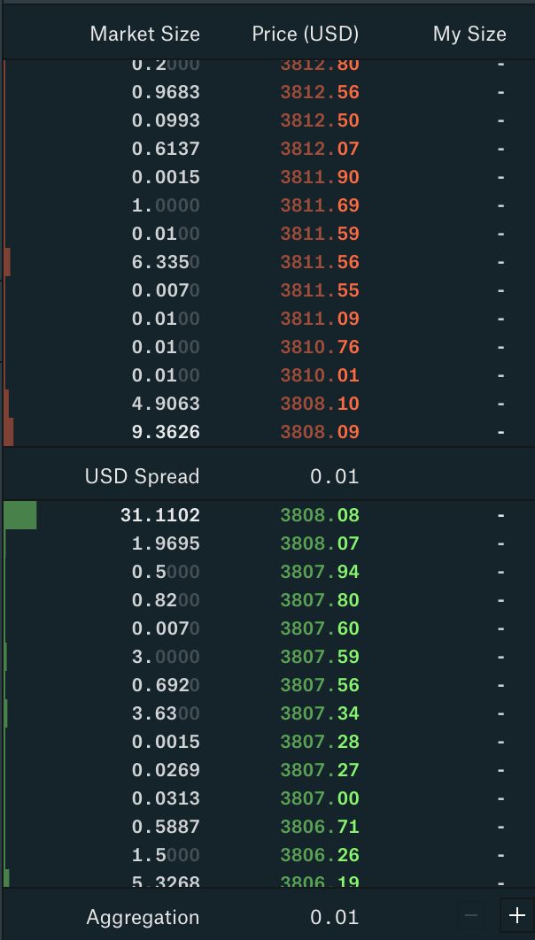
GDAX order book

Secondly, like the tax relationship between producers and consumers, there is a certain degree of equivalence between makers and takers in terms of cost incidence. If you charge the maker relatively more, they will expand the order book and pass some fees on to the taker. If you charge relatively more for the taker, the maker will tighten the order book and absorb some of the maker’s fees.

An extreme case here is that you like maker so much that the order book is squeezed into a jump in price (as we often see on GDAX) and the order book cannot be tightened any more. Based on this, any additional costs will now fall on the exchange itself as a loss of income.

In addition to the extreme example, we can see that it is not important which party collects the fees, but the sum of the fees of the maker and the maker. Finally, like the Laffer Curvein tax policy, the exchange faces the problem of revenue optimization in the charging policy. We can see that the profit income is the same as the tax policy. If the exchange does not charge any fees, they will not get income. If the exchange charges 100% of the fee, there is no transaction, so they have no income. Through some additional research, it is clear that the exchange income at the total cost level is a concave function with a unique maximum.

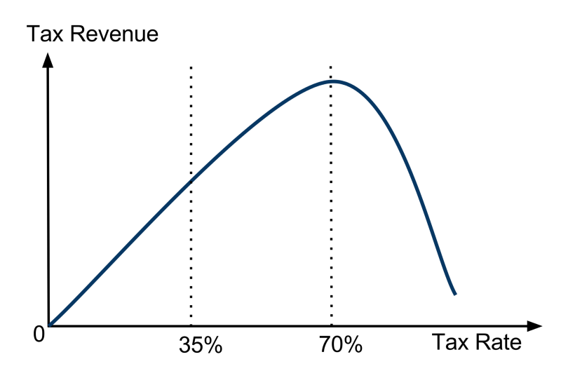
Explanation of the term: Laffer curve (https://en.wikipedia.org/wiki/Laffer_curve)

To be continued…