From Quantitative Trading to Asset Management - CTA Strategy Development for Absolute Return
 0
1408
0
1408
, [nowTime, this.basb]]); ObjChart.add([4, [nowTime, this.sabb]]); ObjChart.update(chart); }
### 4. In the entry function main(), execute the pre-transaction pre-processing code, which will only run once after the program is started, including:

- ```SetErrorFilter ( )``` to filter the unimportant information in the console
- ```exchange.IO ( )``` to set the digital currency to be traded
- ```ObjChart.reset ( )``` to clear the previous chart drawn before starting the program
- ```LogProfitReset ( )``` to clear the status bar information before starting the program

After the above pre-transaction pre-processing is defined, the next step is to enter the polling mode and execute the onTick() function repeatedly. It also sets the sleep time for Sleep () polling, because the API of some digital currency exchanges has built-in access limit for a certain period of time.
function main() { // Filter the unimportant information in the console SetErrorFilter(“429|GetRecords:|GetOrders:|GetDepth:|GetAccount|:Buy|Sell|timeout|Futures_OP”); exchange.IO(“currency”, name + ‘_USDT’); // Set the digital currency to be traded ObjChart.reset(); // Clear the previous chart drawn before starting the program LogProfitReset(); // Clear the status bar information before starting the program while (true) { // Enter the polling mode onTick(); // Execute onTick function Sleep(500); // Sleep for 0.5 seconds } }
## II. Get and calculate data

1. Obtain basic data object, account balance, and boll indicator data for use in the trading logic.
function onTick() { var data = new Data(tradeTypeA, tradeTypeB); // Create a basic data object var accountStocks = data.accountData.Stocks; // Account balance var boll = data.boll(dataLength, timeCycle); // Get boll indicator data if (!boll) return; // Return if there is no boll data }
## III. Place an order and handle the follow-up

1. Execute the buying and selling operation according to the above strategic logic. First, judge whether the price and indicator conditions are valid, then judge whether the position conditions are valid, and finally execute the trade () order function.
// Explanation of the price difference // basb = (Sell one price of contract A - Buy one price of contract B) // sabb = (Buy one price of contract A - Sell one price of contract B) if (data.sabb > boll.middle && data.sabb < boll.up) { // If sabb is higher than the middle track if (data.mp(tradeTypeA, 0)) { // Check whether contract A has long orders before placing an order data.trade(tradeTypeA, “closebuy”); // Contract A closes long position } if (data.mp(tradeTypeB, 1)) { // Check whether contract B has short orders before placing an order data.trade(tradeTypeB, “closesell”); // Contract B closes short position } } else if (data.basb < boll.middle && data.basb > boll.down) { // If basb is lower than the middle track if (data.mp(tradeTypeA, 1)) { // Check whether contract A has short orders before placing an order data.trade(tradeTypeA, “closesell”); // Contract A closes short position } if (data.mp(tradeTypeB, 0)) { // Check whether contract B has long orders before placing an order data.trade(tradeTypeB, “closebuy”); // Contract B closes long position } } if (accountStocks * Math.max(data.askA, data.askB) > 1) { // If there is balance in the account if (data.basb < boll.down) { // If basb price difference is lower than the down track if (!data.mp(tradeTypeA, 0)) { // Check whether contract A has long orders before placing an order data.trade(tradeTypeA, “buy”); // Contract A opens long position } if (!data.mp(tradeTypeB, 1)) { // Check whether contract B has short orders before placing an order data.trade(tradeTypeB, “sell”); // Contract B opens short position } } else if (data.sabb > boll.up) { // If sabb price difference is higher than the upper track if (!data.mp(tradeTypeA, 1)) { // Check whether contract A has short orders before placing an order data.trade(tradeTypeA, “sell”); // Contract A opens short position } if (!data.mp(tradeTypeB, 0)) { // Check whether contract B has long orders before placing an order data.trade(tradeTypeB, “buy”); // Contract B opens long position } } }
2. After the order is placed, it is necessary to deal with the abnormal situations such as the unsettled order and the holding of a single contract. And draw the chart.
data.cancelOrders(); // cancel orders data.drawingChart(boll); // drawing data.isEven(); // Handle holding individual contracts
As above, we have created a simple cross-period arbitrage strategy of digital currency completely through more than 200 lines code. The complete code is as follows:
// Global variable // Declare a chart object for the configuration chart var chart = { __isStock: true, tooltip: { xDateFormat: ‘%Y-%m-%d %H:%M:%S, %A’ }, title: { text: ‘transaction profit and loss curve (detailed)’ }, rangeSelector: { buttons: [{ type: ‘hour’, count: 1, text: ‘1h’ }, { type: ‘hour’, count: 2, text: ‘3h’ }, { type: ‘hour’, count: 8, text: ‘8h’ }, { type: ‘all’, text: ‘All’ }], selected: 0, inputEnabled: false }, xAxis: { type: ‘datetime’ }, yAxis: { title: { text: ‘price difference’ }, opposite: false, }, series: [{ name: “upper track”, id: “line1,up”, data: [] }, { name: “middle track”, id: “line2,middle”, data: [] }, { name: “down track”, id: “line3,down”, data: [] }, { name: “basb”, id: “line4,basb”, data: [] }, { name: “sabb”, id: “line5,sabb”, data: [] }] }; var ObjChart = Chart(chart); // Drawing object var bars = []; // Storage price difference series var oldTime = 0; // Record historical data timestamp
// Parameters var tradeTypeA = “this_week”; // Arbitrage A contract var tradeTypeB = “quarter”; // Arbitrage B contract var dataLength = 10; // Indicator period length var timeCycle = 1; // K-line period var name = “ETC”; // Currencies var unit = 1; // Order quantity
// basic data function Data(tradeTypeA, tradeTypeB) { // Pass in arbitrage A contract and arbitrage B contract this.accountData = _C(exchange.GetAccount); // Get account information this.positionData = _C(exchange.GetPosition); // Get position information var recordsData = _C(exchange.GetRecords); // Get K-line data exchange.SetContractType(tradeTypeA); // Subscribe to arbitrage A contract var depthDataA = _C(exchange.GetDepth); // Arbitrage A contract depth data exchange.SetContractType(tradeTypeB); // Subscribe to arbitrage B contract var depthDataB = _C(exchange.GetDepth); // Arbitrage B contract depth data this.time = recordsData[recordsData.length - 1].Time; // Time to get the latest data this.askA = depthDataA.Asks[0].Price; // Sell one price of arbitrage A contract this.bidA = depthDataA.Bids[0].Price; // Buy one price of arbitrage A contract this.askB = depthDataB.Asks[0].Price; // Sell one price of arbitrage B contract this.bidB = depthDataB.Bids[0].Price; // Buy one price of arbitrage B contract // Positive arbitrage price difference (Sell one price of contract A - Buy one price of contract B) this.basb = depthDataA.Asks[0].Price - depthDataB.Bids[0].Price; // Negative arbitrage price difference (Buy one price of contract A - Sell one price of contract B) this.sabb = depthDataA.Bids[0].Price - depthDataB.Asks[0].Price; }
// Get position Data.prototype.mp = function (tradeType, type) { var positionData = this.positionData; // Get position information for (var i = 0; i < positionData.length; i++) { if (positionData[i].ContractType == tradeType) { if (positionData[i].Type == type) { if (positionData[i].Amount > 0) { return positionData[i].Amount; } } } } return false; }
// Synthesis of new K-line data and boll indicator data Data.prototype.boll = function (num, timeCycle) { var self = {}; // Temporary objects // Median value of between positive arbitrage price difference and negative arbitrage price difference self.Close = (this.basb + this.sabb) / 2; if (this.timeA == this.timeB) { self.Time = this.time; } // Compare two depth data timestamps if (this.time - oldTime > timeCycle * 60000) { bars.push(self); oldTime = this.time; } // Pass in the price difference data object into the K-line array according to the specified time period if (bars.length > num * 2) { bars.shift(); // Control the length of the K-line array } else { return; } var boll = TA.BOLL(bars, num, 2); // Call the boll indicator in the talib library return { up: boll[0][boll[0].length - 1], // boll indicator upper track middle: boll[1][boll[1].length - 1], // boll indicator middle track down: boll[2][boll[2].length - 1] // boll indicator down track } // Return a processed boll indicator data }
// Place an order Data.prototype.trade = function (tradeType, type) { exchange.SetContractType(tradeType); // Resubscribe to a contract before placing an order var askPrice, bidPrice; if (tradeType == tradeTypeA) { // If the order is placed in contract A askPrice = this.askA; // Set askPrice bidPrice = this.bidA; // Set bidPrice } else if (tradeType == tradeTypeB) { // If the order is placed in contract B askPrice = this.askB; // Set askPrice bidPrice = this.bidB; // Set bidPrice } switch (type) { // Match order placement mode case “buy”: exchange.SetDirection(type); // Set order placement mode return exchange.Buy(askPrice, unit); case “sell”: exchange.SetDirection(type); // Set order placement mode return exchange.Sell(bidPrice, unit); case “closebuy”: exchange.SetDirection(type); // Set order placement mode return exchange.Sell(bidPrice, unit); case “closesell”: exchange.SetDirection(type); // Set order placement mode return exchange.Buy(askPrice, unit); default: return false; } }
// Cancel orders Data.prototype.cancelOrders = function () { Sleep(500); // Delay before cancellation, because some exchanges, you know what I mean var orders = _C(exchange.GetOrders); // Get an array of unfilled orders if (orders.length > 0) { // If there are unfilled orders for (var i = 0; i < orders.length; i++) { // Iterate through the array of unfilled orders exchange.CancelOrder(orders[i].Id); // Cancel unfilled orders one by one Sleep(500); // Sleep for 0.5 seconds } return false; // Return false if an unfilled order is cancelled } return true; // Return true if there are no unfilled orders }
// Handle holding individual contracts Data.prototype.isEven = function () { var positionData = this.positionData; // Get position information var type = null; // Switch position direction // If the remaining 2 of the position array length is not equal to 0 or the position array length is not equal to 2 if (positionData.length % 2 != 0 || positionData.length != 2) { for (var i = 0; i < positionData.length; i++) { // Iterate through the position array if (positionData[i].Type == 0) { // If it is a long order type = 10; // Set order parameters } else if (positionData[i].Type == 1) { // If it is a short order type = -10; // Set order parameters } // Close all positions this.trade(positionData[i].ContractType, type, positionData[i].Amount); } } }
// Drawing Data.prototype.drawingChart = function (boll) { var nowTime = new Date().getTime(); ObjChart.add([0, [nowTime, boll.up]]); ObjChart.add([1, [nowTime, boll.middle]]); ObjChart.add([2, [nowTime, boll.down]]); ObjChart.add([3, [nowTime, this.basb]]); ObjChart.add([4, [nowTime, this.sabb]]); ObjChart.update(chart); }
// Trading conditions function onTick() { var data = new Data(tradeTypeA, tradeTypeB); // Create a basic data object var accountStocks = data.accountData.Stocks; // Account balance var boll = data.boll(dataLength, timeCycle); // Get boll indicator data if (!boll) return; // Return if there is no boll data // Explanation of price difference // basb = (Sell one price of contract A - Buy one price of contract B) // sabb = (Buy one price of contract A - Sell one price of contract B) if (data.sabb > boll.middle && data.sabb < boll.up) { // If sabb is higher than the middle track if (data.mp(tradeTypeA, 0)) { // Check whether contract A has long orders before placing an order data.trade(tradeTypeA, “closebuy”); // Contract A closes long position } if (data.mp(tradeTypeB, 1)) { // Check whether contract B has short orders before placing an order data.trade(tradeTypeB, “closesell”); // Contract B closes short position } } else if (data.basb < boll.middle && data.basb > boll.down) { // If basb is lower than the middle track if (data.mp(tradeTypeA, 1)) { // Check whether contract A has short orders before placing an order data.trade(tradeTypeA, “closesell”); // Contract A closes short position } if (data.mp(tradeTypeB, 0)) { // Check whether contract B has long orders before placing an order data.trade(tradeTypeB, “closebuy”); // Contract B closes long position } } if (accountStocks * Math.max(data.askA, data.askB) > 1) { // If there is a balance in the account if (data.basb < boll.down) { // If basb price difference is lower than the down track if (!data.mp(tradeTypeA, 0)) { // Check whether contract A has long orders before placing an order data.trade(tradeTypeA, “buy”); // Contract A opens long position } if (!data.mp(tradeTypeB, 1)) { // Check whether contract B has short orders before placing an order data.trade(tradeTypeB, “sell”); // Contract B opens short position } } else if (data.sabb > boll.up) { // If sabb price difference is higher than the upper track if (!data.mp(tradeTypeA, 1)) { // Check whether contract A has short orders before placing an order data.trade(tradeTypeA, “sell”); // Contract A opens short position } if (!data.mp(tradeTypeB, 0)) { // Check whether contract B has long orders before placing an order data.trade(tradeTypeB, “buy”); // Contract B opens long position } } } data.cancelOrders(); // Cancel orders data.drawingChart(boll); // Drawing data.isEven(); // Handle holding individual contracts }
// Entry function function main() { // Filter unimportant information in the console SetErrorFilter(“429|GetRecords:|GetOrders:|GetDepth:|GetAccount|:Buy|Sell|timeout|Futures_OP”); exchange.IO(“currency”, name + ‘_USDT’); //Set the digital currency to be traded ObjChart.reset(); // Clear the previous chart drawn before starting the program LogProfitReset(); // Clear the status bar information before starting the program while (true) { // Enter polling mode onTick(); // Execute the onTick function Sleep(500); // Sleep for 0.5 seconds } } “` Arbitrage trading originated from the stock trading strategy of Morgan Stanley. Its idea is that the price difference of two highly correlated varieties conforms to the “popcorn process”, that is, the price difference keeps returning to the mean from a position that deviates from the historical mean, and then deviates again from the mean.
Therefore, we can buy low and sell high on the price difference to gain profits. Then, according to the principle of standard deviation in statistics, the Bollinger band is formed by a middle track and the upper and lower tracks calculated by the standard deviation, the formation of three mesh band, which are very practical in the price difference arbitrage transaction.
After testing, operating according to this strategy, the overall income is relatively stable, although the income is not very much each time without considering the handling fee and impact cost. It should be noted that due to the statistical arbitrage, there is a risk of reverse expansion of the price difference. We must consider the stop-loss problem when designing. Secondly, we also need to pay attention to the impact cost. When the liquidity of the two contracts involved in the transaction shrinks, it will have a great impact on the income, and investors should avoid it as appropriate.
4. Advanced iteration of CTA strategy development
4.1 Avoid the pitfalls of futures CTA strategy
In the last two classes, we wrote a trend strategy in MyLanguage and an arbitrage strategy in JavaScript. We didn’t see any problems in the strategy backtest. However, quantitative trading is not a program, whose backtest can be done directly without any problems.
In fact, the backtest is only a simulation of the strategy. It is only used to evaluate the performance of the strategy in the historical data. It allows traders to evaluate and discard some trading strategies quickly.
In many cases, strategies that look great in the backtest often fail to meet the backtest standard in the real market for a variety of reasons. Some of them are beyond the control of traders, but some of the failures are caused by common or potential errors.
Static data and dynamic data
We should have a concept of static data and dynamic data to quantify first. In the backtest, we use static historical data. The price of opening high and closing low with each K-line is complete, and each transaction signal can be closed 100%. But the data in the real market is dynamic. For example, if the maximum price is greater than the maximum price within 1 hour of opening, buy. But if the current K-line has not finished, the maximum price is dynamic, and the trading signal may flicker back and forth. This situation indicates that the strategy uses the future function in judging the conditions of the buy and sell trading.
Future function
What is the future function? Let’s take a look at Baidu Encyclopedia’s explanation first: A quantity depends on another quantity, such as quantity A and quantity B. If B changes, A changes, then A is a function of B. If B is a later quantity, A is an earlier quantity, A changes with B, and A is a future function of B. You may be confused.
Generally speaking, it is a function of quoting future data, such as forecasting tomorrow’s price with tomorrow’s price. If a technical indicator contains a future function, its signal is uncertain. It is often the current transaction signal. When the next K-line appears, the signal disappears or changes position.
The closing price is a future function. The closing price is always changing until the latest K-line runs out. You must wait until the K-line runs out to determine the closing price. Since the closing price itself is a future function, all technical indicators based on the closing price are also future functions.
Therefore, if a technical indicator uses the confirmed closing price as the basic data, the trading signal will not change no matter how long it has passed, it can be said that the technical indicator does not refer to the future function. But the basic data it uses is the unconfirmed closing price, so this technical indicator refers to the future function, and the trading signal may change in practical application.
Past prices
The future function uses the future price, which may also use the past price on the contrary. This is also a problem that many novices tend to ignore. To better illustrate this problem in the future, let’s take an example: if the current maximum price is greater than the maximum price within 1 hour after the opening, buy at the opening price. Obviously, there is no problem with the conditions of the buying and selling signal, but the price of the order has used the past price.
In the backtest, the strategy is normal, because the backtest engine based on static data can be closed 100% only if there is a buy signal. However, when the highest price is greater than the highest price within 1 hour after the opening, it is certain that the order cannot be issued at the previous price opening price.
Price vacuum
The so-called price vacuum refers to the prices displayed on the K-line chart, but the prices that cannot be traded in the real market, mainly divided into the following cases:
- 1. Anyone who has done trading knows that it is difficult to buy when the price is up and difficult to sell when the price is down. But it can be concluded in the backtest.
- 2. The matching mechanism of the exchange is price priority and time priority. Some varieties will often have a large number of orders in the market. If you are trading with orders in the real market, you must rank behind others’ orders. You can only trade after others’ orders are traded. Even before the price can be traded, the price has changed. However, in the backtest, if your strategy is to deal with the order, you will deal in time, which is different from the real market environment.
- 3. If you use an arbitrage strategy, the profit of the backtest is very high, because it is assumed that you have captured these price differences every time. In reality, many price differentials can’t be grabbed, or only one leg can be grabbed. Generally speaking, it must be the one that is not conducive to your direction. Then you need to fill the other leg immediately. At this time, the sliding point is no longer 1 or 2 points, and the arbitrage strategy itself aims to earn the price difference of these points. This situation cannot be simulated in the backtest. The real profit is not as good as the backtest.
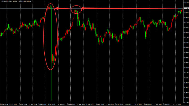
- 4. Although the black swan event is not used commonly, it still has a great impact on quantitative trading. As shown in the chart below, in the case of the black swan event of the foreign exchange Swiss franc, both high and low prices can be seen from the chart. In fact, in the extreme market of the day, the middle price is vacuum, and a large number of stop loss orders cause stampede events. The liquidity is zero, and it is very difficult to deal with, but it can stop loss in the backtest.
Overfitting
Overfitting is a common mistake made by quantitative trading beginners. What is overfitting? To take a simple example, some people use a great deal of exercises to memorize each question in the school exam. He can’t do it if the subject changes a little during the exam. Because he memorized the practice of each question in a very complex way, he did not abstract the general rules.
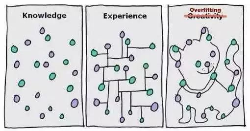
Like the chart above, a model can adapt to data perfectly as long as it is complex enough. This is also true of overfitting in quantitative trading. If your strategy is complex and it has many external parameters, there will always be one or several parameters that can perfectly fit the historical market in the limited historical data backtest.
However, in the future real market, the price change may exceed your strategy limit. In fact, the essence of quantitative trading strategy development is the process of matching local non-random data from a large number of seemingly random data. Therefore, we need to use statistical knowledge to avoid the trap. How do we do it?
The compromise solution is to use intra-sample and extra-sample data. Divide the whole data into two parts, and use the intra-sample as the training set, which is responsible for the data backtest. The extra-sample is used as the test set and is responsible for verification. If there is little historical data, you can also use the cross-test method.
If you find that the data out of the sample performs not well, and you feel that it is too bad to lose the model or you are unwilling to admit that your model is not good, and you continue to optimize the model for the extra-sample data until the extra-sample data also perform well, then you must lose your money in the end.
Survivorship bias
The survivorship bias can be explained by the following examples: 1. When standing at the tuyere, pigs will fly. 2. People who sell parachutes online are praised, because people with problems with parachutes don’t live anymore. 3. The reporter interviewed whether passengers have bought tickets on the bus, because people without tickets can’t get on the bus at all. 4. The media advertises that the lottery can be won, because the media will not actively promote people who do not win the lottery.
In the above example, we can find that the information that people usually receive is actually filtered, which makes a large number of data or samples ignored selectively, and the result is that the conclusions based on survivorship bias have deviated from real-time. So in quantitative trading, we also need to focus on whether the results of the backtest are part of luck. In many cases, the results of the backtest may be the best performance in the whole backtest. Pay attention to the following figure:
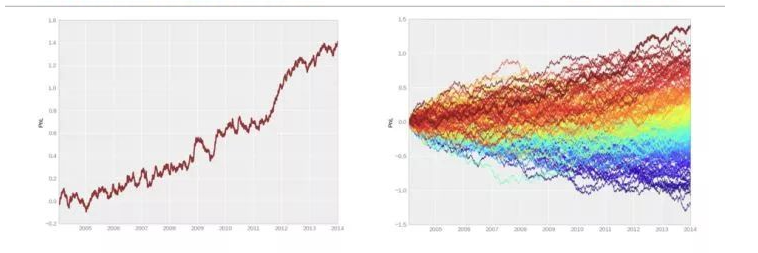
- Left chart (semblance): A very good trading strategy. Without major withdrawal, investors can obtain stable investment returns.
- Right chart (the reality): This is only the best one in 200 random trading backtests.
The picture on the left is a very good trading strategy. The capital curve is good, and there is no significant withdrawal, and stable profit returns can be obtained. But look at the picture on the right. It is only the best one in the hundreds of backtest transactions. On the other hand, when we look at the financial market, there are always more stars and less longevity stars. If the strategy of the traders is consistent with the market situation, then the market every year can create a batch of stars, but it is difficult to see longevity stars who can make steady profits for more than three years in a row.
Cost shock
Unless you are pending an order, you may have a sliding price when trading. On the varieties with active trading, the bid-price and ask-price are usually different in one point. On the varieties with inactive trading, the difference may be greater. Every time you want to take the initiative to close a deal, you need one point difference at least, or even more. However, in the backtest, we do not need to consider the issue of transaction, as long as there is a signal, we can trade, so in order to simulate the real trading environment, we must add one sliding price at least.
Especially for the strategy that is traded more frequently, if the sliding price is not added when the strategy is backtested, the capital curve will always tilt upward, and once the reasonable sliding price is added, it will turn to a loss immediately. In addition, this phenomenon is not only caused by point difference, but also needs to be considered in the real trading environment: network delay, software and hardware systems, server response and other issues.
Strategy capacity
The same strategy will be quite different in efficient and inefficient markets, even the opposite. For example, in inefficient markets such as domestic stock markets, commodity futures, and foreign digital currencies, due to the small base of trading volume, the capacity of high-frequency strategy itself is not very large, and there is no profit space for more people, and even the strategy that was originally profitable has become a loss. But in an efficient foreign exchange market, it can accommodate many different types of high-frequency strategies.
The above are the problems and pitfalls that may occur in the development and use of strategies. For an experienced trading system developer, backtesting is a must. Because it can tell you whether a strategic idea can be verified in historical transactions. But many times, backtesting does not mean that it will be profitable in the future. Because there are too many pitfalls in the backtest, you won’t understand without paying for some lessons. This course can help you avoid many quantitative detours and pitfalls at least.
4.2 Establish the best position management
In “Reminiscences of a stock operator”, there is a very interesting paragraph: the Old Turkey (formerly known as Partridge) who is in the same securities company as the hero Livermore, always makes a big deal. When he was advised to sell after taking profits and buy again after the stock price had retraced. The Old Turkey always intoned: No, you know, this is a bull market!
Even Livermore sighed finally: There is nothing remarkable about the trend. There are always many people who are bullish in the bull market and bearish in the bear market. But they are always good at bargaining with the market, trying to buy at the lowest point and sell at the highest point. Like the Old Turkey, it is those who see the market and hold their positions that really make a great fortune, which is also the most difficult to learn. This not only faces the choice of target and timing, but also faces a more important question: how much position (risk) should we hold (bear)?
All failed traders have one-sided thinking. When trading, greedy people only see profits rather than risks, while timid people only see risks rather than profits. Greedy and timid people forget risks when rising, and forget profits when falling. However, successful traders will consider both risks and returns, that is to say, they will bear several dollars of risk for every dollar they earn. Then the index to measure return and risk is the return risk ratio.
Many people know that the risk is as big as the profit, that is, the return is proportional to the risk. In the view of some people, the relationship between return and risk should be as follows: the horizontal axis is the percentage of risk, and the vertical axis is the percentage of return:
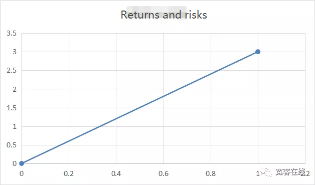
But in the actual transaction, the return and risk are far from being as simple as two points of a line, at least it doesn’t always move linearly. The real risk is the maximum amount of loss that can be taken with the expected return, or what we call the maximum volatility. Although sometimes the maximum floating loss does not always equal the closing loss in terms of the outcome of the trade, the maximum floating loss is real.
From this, we can know that the ratio of return to risk in the figure above is not the real performance. In a real trading environment, the ratio of return to risk should be the same as in the chart below:
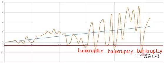
Let’s look at the chart above. The yellow curve shows the fluctuation of net worth at different risks. With the expected returns expanding, the risks are also expanding gradually. If we set bankruptcy at 0.5, that is, the maximum loss reaches 50%, then this is a failed trading strategy. Although the final return of the strategy is positive from the result, it has already gone bankrupt in the middle.
Even if your strategy is a positive one, it will be liquidations under the wrong position management. So from this point of view, how much to buy and sell is more important than when to buy and sell. How to manage the position scientifically has become a fundamental issue in financial transactions. So before trying to solve this problem, let’s see how to bet scientifically in gambling.

Let’s take the coin toss as an example. Suppose that both sides of a coin are equally weighted. If there is a head profit of 2 yuan and a tail loss of 1 yuan, it is obvious that this is a positive expectation game. The winning rate is 50% and a loss of 2. Here comes the question: Now that you have 100 yuan, how can you repeat the bet so that 100 yuan can reach 1 million yuan at the fastest speed.
If we don’t think carefully, we will think that since the return of each bet is 50% * 2-50% * 1, that is, 50%, then in order to achieve the maximum return quickly, we should invest as much capital as possible in each bet. This bet must be 100%.
However, it is obvious that it is unreasonable to invest 100% of the principal in every game of gambling, because as long as you lose the principal once, it will be lost, even if it is very unlikely. Because as long as you gamble enough times, losing money will happen definitely.
Someone may ask, since 100% bet is unreasonable, what about 90% or lower bet? In fact, to solve this problem, we can make an experiment to simulate the gambling game and see how the result of each bet is. As shown in the following chart:
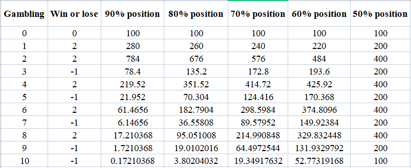
From the chart, we can see that when we gradually reduce the position from 90%, 80%, 70%, 60% and 50%, in the same gamble, the results are completely different. Careful friends may have noticed that with the gradual reduction of the position, the final capital is expanding gradually.
Then some people may ask whether the smaller the bet each time is, the better, such as 10%. It is impossible to calculate every bet proportion. This is the problem to be solved by the famous Kelly Criterion. In statistics, Kelly Criterion can maximize the long-term growth rate of a strategy with positive expectation of repeated bets, and it can calculate the best bet ratio in each bet.
Not only that, assuming that the principal and the bet can be divided endlessly, it is impossible to go bankrupt in any bet by using the Kelly Criterion. Especially in the practical application of financial transactions, it is a position management strategy with both attack and defense. Let’s look at how Kelly Criterion is calculated, and see the following figure:
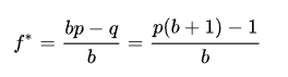
- f is the optimal betting ratio for the available capital;
- b is the odds ratio, which can also be called the profit/loss ratio in trading;
- p is the success rate;
- q is the failure rate.
Then we can calculate the gambling example in this lesson according to the Kelly Criterion. The initial capital of 100 yuan can reach 1 million yuan at the fastest speed by using the betting ratio when the winning ratio is 50% and the odds is 2. Set into the Kelly Criterion, the calculation process is as follows:
(0.5*(2+1) -1)/2=0.25
The winning rate of 50% is 0.5. Multiply the odds by 2 plus 1, then subtract 1, and then divide by 2. The calculation result is 0.25. That is to say, in each bet, using 25% of the principal, you can reach 1 million yuan at the fastest speed. We can simulate manually according to the calculation results to see if it is correct.
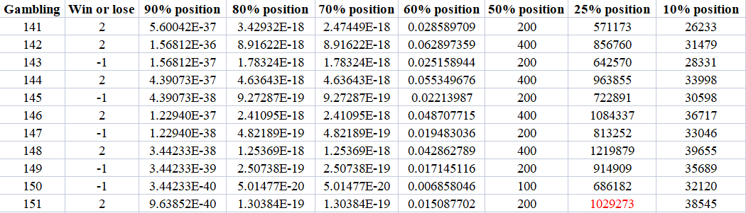
The figure above is the result of manual simulation. Please see the last line. In the same bet, after more than 100 rounds, 25% of the positions reached 1 million yuan first. The result of 90%, 80%, 70% and 60% positions is negative, which shows that even a positive expectation trading strategy will go bankrupt under the wrong position management.
We can also see that 50% of the positions will not lose or win in the end, which is also consistent with the result of the law of large numbers. In order to further illustrate the problem, a position of 10% was also added in the manual simulation. Although the final result was a positive return, the effect was several orders of magnitude worse than that of a position of 25%.
You can see the power of Kelly Criterion. If you choose 10% of the principal position in the actual application, your principal will become more than 30,000 in more than 100 bets. Although the return is large, compared with 25% of the principal position, it is equivalent to no profit. This is the power of knowledge.
If you want to make profits from Kelly Criterion in life, you need to meet the application conditions of Kelly Criterion. There is no doubt that this bet must come from the financial market. Especially in quantitative trading, we can roughly calculate the corresponding winning ratio and odds through historical data backtesting.
Of course, the practical application of Kelly Criterion in financial transactions cannot be so simple, and there are many details to be dealt with, such as the cost of capital in leveraged transactions, the capital and position in real transactions can not be divided wirelessly, and the winning ratio and loss ratio in transactions are changing dynamically, and so on. Whatever, Kelly Criterion shows us how to establish the best position management method.
- Concurrent Strategy Execution with JavaScript Multithreading Support
- 让策略程序真正并发执行,给JavaScript策略增加系统底层多线程支持
- If you don't know how to write a strategy in such an easy-to-learn and easy-to-use Pine language...
- 高频交易的预期收益
- Can we make quantitative trading without code? Let's find out...
- "Get the best deal" analysis of the vulnerability in the exchange
- 5.6 Build probability thinking to improve your trading pattern
- Elegant and simple! Accessed Uniswap V3 on FMZ with 200 lines of code
- When FMZ encounters ChatGPT, an attempt to use AI to assist in learning quantitative trading
- 9 trading rules help a trader earn $46,000 from $1,000 in less than a year
- Create a Bitcoin trading robot that won't lose money
- The Secret to Survival: 19 Professionals Share Their Advice on Digital Currency Trading
- Use JavaScript to implement the concurrent execution of quantitative strategy - encapsulate the Go function
- The Application of "Shannon's Demon" in Digital Currency
- 优雅简洁!在FMZ上用200行代码接入了Uniswap V3
- Principle and compilation of stop-loss model
- Tycoon reveals algorithm trading: FMZ Quant platform market maker strategy
- Three potential models in quantitative trading
- Pivot Point Intraday Trading System
- 6 Simple Strategies and Practices for Beginners in Digital Currency Quantitative Trading