Oscillation Balance Strategy

Overview
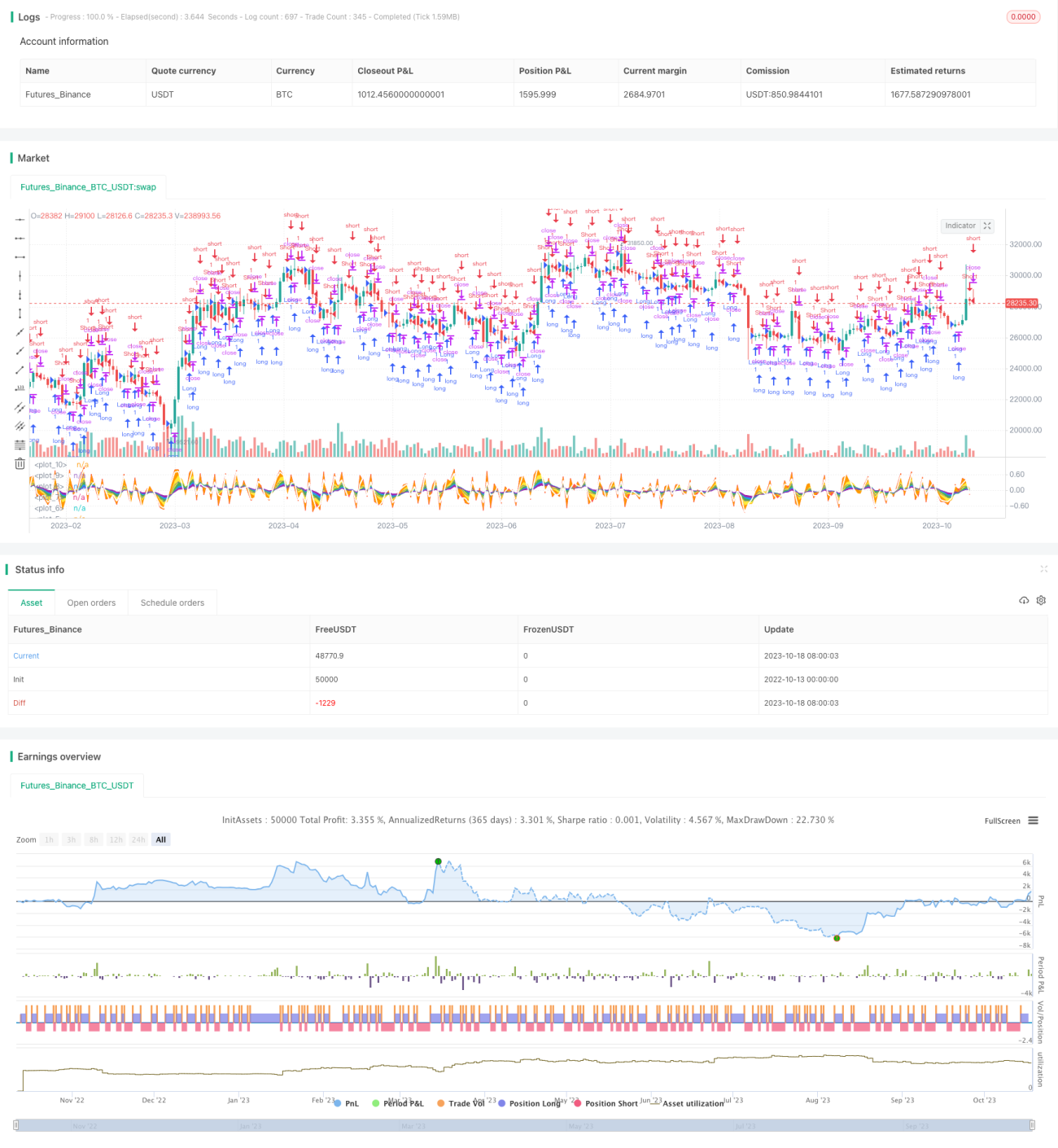
The Oscillation Balance strategy is a simple strategy that uses weighted moving averages and basic lookback periods to predict price movement in the next tick. It calculates the current close position relative to the open based on high and low, then computes exponential moving averages of different periods, and finally judges the general price trend based on historical data.
Principle Analysis
The strategy first calculates the close position relative to open: BoP = (close - open) / (high - low). Then it calculates the EMAs of periods 3, 6, 9, 12, and 18.
Drawing EMAs in different colors shows that shorter period lines change direction first, while longer period lines provide support and resistance. Filling the areas between EMAs makes it more intuitive to see the price oscillation between the lines.
It further takes the arithmetic mean of these EMAs to get a comprehensive line. Looking at the change of this line in the past two periods, it predicts the trend in the next period. If the comprehensive line rises, go long. If it falls, go short.
This way, it estimates a general future trend based on historical data. Although very simple, the visual EMAs and fillings clearly show the price oscillation.
Advantage Analysis
The advantages of this strategy include:
-
The principle is simple and easy to understand and implement.
-
It aggregates complex price history into a simple comprehensive line for judging entry and exit points by direction.
-
The combination of multiple period EMAs provides more comprehensive references. Short period lines determine specific entry while long period ones decide general trend.
-
Filling between EMAs forms an intuitive visual effect for seeing clear price oscillation.
-
No need to set stop loss or take profit, avoiding unnecessary trades.
Risk Analysis
The risks of this strategy include:
-
The prediction is solely based on past data, not ensuring future occurrence. It needs confirmation with trends and key levels.
-
Sudden price changes from events may render inaccurate predictions. Proper risk control is required.
-
Multiple EMAs can generate confused signals. Weights need to be optimized.
-
High trading frequency may happen and interval control is needed to reduce unnecessary trading.
-
The strategy signals lag, possibly causing late entry and premature stop loss.
Optimization Directions
The strategy can be optimized in the following aspects:
-
Optimize the EMA weights for clearer signals. For example, increase weights for medium and long term EMAs.
-
Add trend indicator confirmation to avoid counter trend trades. Such as using ADX to determine trend strength.
-
Add filters at key support and resistance levels to reduce false signals.
-
Optimize entry rules to avoid unnecessary opening positions. Trend filter or volume confirmation can be added.
-
Optimize stop loss methods like curve stop loss or ATR stop loss.
-
Add sentiment indicators to avoid chasing tops and bottoms. For example, long/short ratio and fund flow.
-
Control interval to lower trading frequency. Or optimize number of trades to avoid overtrading.
Summary
The Oscillation Balance strategy judges entry and exit points simply and intuitively by calculating price oscillation and visualizing EMAs of multiple periods. Although risks like prediction lag and wrong signals exist, it can be optimized by adding filters, stop loss methods etc. It provides useful references when trend trading. This strategy suits frequent short-term traders and visual pattern analyzers.
- 1