ANN-based Quantitative Trading Strategy

Author: ChaoZhang, Date: 2023-11-14 11:22:28
Tags:

img

Overview

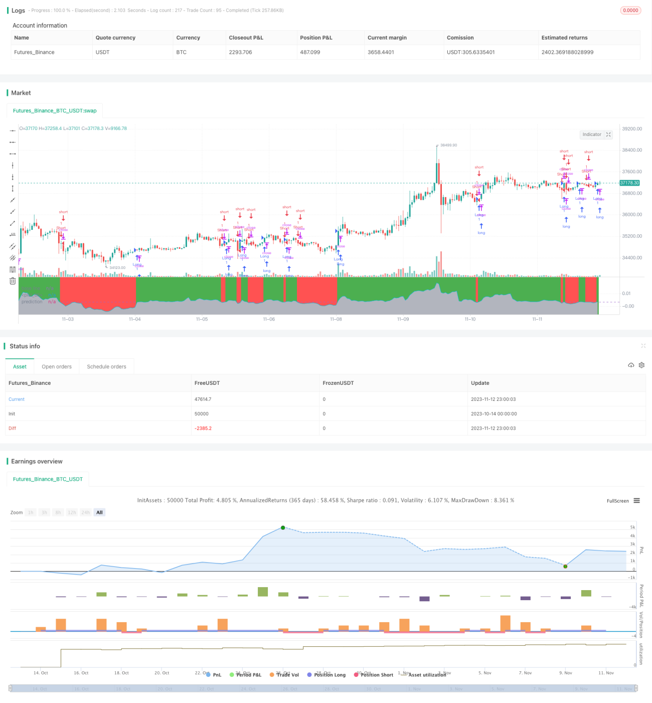
This strategy uses an artificial neural network (ANN) to predict future price changes and generates trading signals based on the predictions. It belongs to the trend following strategy. The advantage is that it can identify complex nonlinear trends and is suitable for medium-to-long term trading. However, it also has the risk of overfitting to backtest data and underperforming in live trading.

Strategy Logic

The strategy uses an ANN model to predict the percentage change of the next trading day.

The input layer has only one node, which is the percentage change of the previous day.

The hidden layer has 2 layers, the first with 5 nodes, and the second with 33 nodes. Both use hyperbolic tangent (tanh) as activation function.

The output layer has one node, going through a linear activation function to generate the final prediction.

If the prediction is greater than the threshold parameter, a long signal is generated. If less than the negative of threshold, a short signal is generated.

Advantages

  • ANN can model complex nonlinear relationships in data
  • Only requires data from previous day as input
  • Can identify longer timeframes trends
  • Multiple hidden layers increase modeling capability
  • Activation functions and parameters optimized for good performance

Risks

  • Overfitting risk - live performance may differ from backtest
  • Requires longer historical data for training
  • Parameters and structure need optimization, results may vary
  • Only predicts next day, unable to determine long term trends
  • Performance may degrade during ranging markets

Improvement Directions

  • Add more input variables like volume etc
  • Try different ANN architectures and activation functions
  • Optimize network parameters for better fit
  • Increase sample size of training data to reduce overfitting
  • Predict across multiple time horizons to better identify trends
  • Ensemble with other models
  • Use volatility measures etc for better risk control

Conclusion

This ANN-based strategy can identify complex nonlinear trends and is suitable for medium-to-long term trading. However, the black-box nature of ANN models also poses significant challenges for live trading. We need to optimize across input features, model architecture, parameter tuning, ensemble learning etc. while combining with traditional technical analysis for robust real-world performance. AI strategies still need to blend with conventional techniques to maximize performance.


/*backtest
start: 2023-10-14 00:00:00
end: 2023-11-13 00:00:00
period: 1h
basePeriod: 15m
exchanges: [{"eid":"Futures_Binance","currency":"BTC_USDT"}]
*/

//@version=2
strategy("ANN Strategy v2")

threshold = input(title="Threshold", type=float, defval=0.0000, step=0.0001)
timeframe = input(title="Timeframe",  defval='1D' )

getDiff() =>
    yesterday=request.security(syminfo.tickerid, timeframe, ohlc4[1])
    today=ohlc4
    delta=today-yesterday
    percentage=delta/yesterday

PineActivationFunctionLinear(v) => v
PineActivationFunctionTanh(v) => (exp(v) - exp(-v))/(exp(v) + exp(-v))


l0_0 = PineActivationFunctionLinear(getDiff())

l1_0 = PineActivationFunctionTanh(l0_0*0.8446488687)
l1_1 = PineActivationFunctionTanh(l0_0*-0.5674069006)
l1_2 = PineActivationFunctionTanh(l0_0*0.8676766445)
l1_3 = PineActivationFunctionTanh(l0_0*0.5200611473)
l1_4 = PineActivationFunctionTanh(l0_0*-0.2215499554)

l2_0 = PineActivationFunctionTanh(l1_0*0.3341657935 + l1_1*-2.0060003664 + l1_2*0.8606354375 + l1_3*0.9184846912 + l1_4*-0.8531172267)
l2_1 = PineActivationFunctionTanh(l1_0*-0.0394076437 + l1_1*-0.4720374911 + l1_2*0.2900968524 + l1_3*1.0653326022 + l1_4*0.3000188806)
l2_2 = PineActivationFunctionTanh(l1_0*-0.559307785 + l1_1*-0.9353655177 + l1_2*1.2133832962 + l1_3*0.1952686024 + l1_4*0.8552068166)
l2_3 = PineActivationFunctionTanh(l1_0*-0.4293220754 + l1_1*0.8484259409 + l1_2*-0.7154087313 + l1_3*0.1102971055 + l1_4*0.2279392724)
l2_4 = PineActivationFunctionTanh(l1_0*0.9111779155 + l1_1*0.2801691115 + l1_2*0.0039982713 + l1_3*-0.5648257117 + l1_4*0.3281705155)
l2_5 = PineActivationFunctionTanh(l1_0*-0.2963954503 + l1_1*0.4046532178 + l1_2*0.2460580977 + l1_3*0.6608675819 + l1_4*-0.8732022547)
l2_6 = PineActivationFunctionTanh(l1_0*0.8810811932 + l1_1*0.6903706878 + l1_2*-0.5953059103 + l1_3*-0.3084040686 + l1_4*-0.4038498853)
l2_7 = PineActivationFunctionTanh(l1_0*-0.5687101164 + l1_1*0.2736758588 + l1_2*-0.2217360382 + l1_3*0.8742950972 + l1_4*0.2997583987)
l2_8 = PineActivationFunctionTanh(l1_0*0.0708459913 + l1_1*0.8221730616 + l1_2*-0.7213265567 + l1_3*-0.3810462836 + l1_4*0.0503867753)
l2_9 = PineActivationFunctionTanh(l1_0*0.4880140595 + l1_1*0.9466627196 + l1_2*1.0163097961 + l1_3*-0.9500386514 + l1_4*-0.6341709382)
l2_10 = PineActivationFunctionTanh(l1_0*1.3402207103 + l1_1*0.0013395288 + l1_2*3.4813009133 + l1_3*-0.8636814677 + l1_4*41.3171047132)
l2_11 = PineActivationFunctionTanh(l1_0*1.2388217292 + l1_1*-0.6520886912 + l1_2*0.3508321737 + l1_3*0.6640560714 + l1_4*1.5936220597)
l2_12 = PineActivationFunctionTanh(l1_0*-0.1800525171 + l1_1*-0.2620989752 + l1_2*0.056675277 + l1_3*-0.5045395315 + l1_4*0.2732553554)
l2_13 = PineActivationFunctionTanh(l1_0*-0.7776331454 + l1_1*0.1895231137 + l1_2*0.5384918862 + l1_3*0.093711904 + l1_4*-0.3725627758)
l2_14 = PineActivationFunctionTanh(l1_0*-0.3181583022 + l1_1*0.2467979854 + l1_2*0.4341718676 + l1_3*-0.7277619935 + l1_4*0.1799381758)
l2_15 = PineActivationFunctionTanh(l1_0*-0.5558227731 + l1_1*0.3666152536 + l1_2*0.1538243225 + l1_3*-0.8915928174 + l1_4*-0.7659355684)
l2_16 = PineActivationFunctionTanh(l1_0*0.6111516061 + l1_1*-0.5459495224 + l1_2*-0.5724238425 + l1_3*-0.8553500765 + l1_4*-0.8696190472)
l2_17 = PineActivationFunctionTanh(l1_0*0.6843667454 + l1_1*0.408652181 + l1_2*-0.8830470112 + l1_3*-0.8602324935 + l1_4*0.1135462621)
l2_18 = PineActivationFunctionTanh(l1_0*-0.1569048216 + l1_1*-1.4643247888 + l1_2*0.5557152813 + l1_3*1.0482791924 + l1_4*1.4523116833)
l2_19 = PineActivationFunctionTanh(l1_0*0.5207514017 + l1_1*-0.2734444192 + l1_2*-0.3328660936 + l1_3*-0.7941515963 + l1_4*-0.3536051491)
l2_20 = PineActivationFunctionTanh(l1_0*-0.4097807954 + l1_1*0.3198619826 + l1_2*0.461681627 + l1_3*-0.1135575498 + l1_4*0.7103339851)
l2_21 = PineActivationFunctionTanh(l1_0*-0.8725014237 + l1_1*-1.0312091401 + l1_2*0.2267643037 + l1_3*-0.6814258121 + l1_4*0.7524828703)
l2_22 = PineActivationFunctionTanh(l1_0*-0.3986855003 + l1_1*0.4962556631 + l1_2*-0.7330224516 + l1_3*0.7355772164 + l1_4*0.3180141739)
l2_23 = PineActivationFunctionTanh(l1_0*-1.083080442 + l1_1*1.8752543187 + l1_2*0.3623326265 + l1_3*-0.348145191 + l1_4*0.1977935038)
l2_24 = PineActivationFunctionTanh(l1_0*-0.0291290625 + l1_1*0.0612906199 + l1_2*0.1219696687 + l1_3*-1.0273685429 + l1_4*0.0872219768)
l2_25 = PineActivationFunctionTanh(l1_0*0.931791094 + l1_1*-0.313753684 + l1_2*-0.3028724837 + l1_3*0.7387076712 + l1_4*0.3806140391)
l2_26 = PineActivationFunctionTanh(l1_0*0.2630619402 + l1_1*-1.9827996702 + l1_2*-0.7741413496 + l1_3*0.1262957444 + l1_4*0.2248777886)
l2_27 = PineActivationFunctionTanh(l1_0*-0.2666322362 + l1_1*-1.124654664 + l1_2*0.7288282621 + l1_3*-0.1384289204 + l1_4*0.2395966188)
l2_28 = PineActivationFunctionTanh(l1_0*0.6611845175 + l1_1*0.0466048937 + l1_2*-0.1980999993 + l1_3*0.8152350927 + l1_4*0.0032723211)
l2_29 = PineActivationFunctionTanh(l1_0*-0.3150344751 + l1_1*0.1391754608 + l1_2*0.5462816249 + l1_3*-0.7952302364 + l1_4*-0.7520712378)
l2_30 = PineActivationFunctionTanh(l1_0*-0.0576916066 + l1_1*0.3678415302 + l1_2*0.6802537378 + l1_3*1.1437036331 + l1_4*-0.8637405666)
l2_31 = PineActivationFunctionTanh(l1_0*0.7016273068 + l1_1*0.3978601709 + l1_2*0.3157049654 + l1_3*-0.2528455662 + l1_4*-0.8614146703)
l2_32 = PineActivationFunctionTanh(l1_0*1.1741126834 + l1_1*-1.4046408959 + l1_2*1.2914477803 + l1_3*0.9904052964 + l1_4*-0.6980155826)

l3_0 = PineActivationFunctionTanh(l2_0*-0.1366382003 + l2_1*0.8161960822 + l2_2*-0.9458773183 + l2_3*0.4692969576 + l2_4*0.0126710629 + l2_5*-0.0403001012 + l2_6*-0.0116244898 + l2_7*-0.4874816289 + l2_8*-0.6392241448 + l2_9*-0.410338398 + l2_10*-0.1181027081 + l2_11*0.1075562037 + l2_12*-0.5948728252 + l2_13*0.5593677345 + l2_14*-0.3642935247 + l2_15*-0.2867603217 + l2_16*0.142250271 + l2_17*-0.0535698019 + l2_18*-0.034007685 + l2_19*-0.3594532426 + l2_20*0.2551095195 + l2_21*0.4214344983 + l2_22*0.8941621336 + l2_23*0.6283377368 + l2_24*-0.7138020667 + l2_25*-0.1426738249 + l2_26*0.172671223 + l2_27*0.0714824385 + l2_28*-0.3268182144 + l2_29*-0.0078989755 + l2_30*-0.2032828145 + l2_31*-0.0260631534 + l2_32*0.4918037012)

buying = l3_0 > 0 ? true : l3_0 < -0 ? false : buying[1]

hline(0, title="base line")
//bgcolor(l3_0 > 0.0014 ? green : l3_0 < -0.0014 ? red : gray, transp=20)
bgcolor(buying ? green : red, transp=20)
plot(l3_0, color=silver, style=area, transp=75)
plot(l3_0, color=aqua, title="prediction")

longCondition = buying
if (longCondition)
    strategy.entry("Long", strategy.long)

shortCondition = buying != true
if (shortCondition)
    strategy.entry("Short", strategy.short)

More