Trend Breakout Strategy Based on Bollinger Bands

Overview
This is a trend following strategy based on Bollinger Bands. It uses Bollinger Bands to calculate price channels and combines candlestick patterns to determine trend direction. Long/short positions will be opened when price breaks out of the Bollinger Bands. This strategy works well for stocks with obvious trends and aims to capture mid-term trend profits.
Strategy Logic
This strategy uses the upper band, middle band and lower band of Bollinger Bands to determine price ranges. The upper and lower bands envelope price movements while the middle band is the moving average. Band width changes based on price volatility. When price breaks above the upper band, it signals an upward breakout and a long entry. When price breaks below the lower band, it signals a downward breakout and a short entry.
After determining trend direction with Bollinger Bands breakout, the strategy also confirms it with candlestick patterns. If the candle body aligns with the trend, such as bullish candle in an uptrend, a position will be opened. If the candle body shows reverse pattern, such as bearish candle in an uptrend, the signal will be ignored. This design aims to avoid false breakout risks.
The detailed trading signals rules are:
-
Calculate upper band, middle band and lower band of Bollinger Bands to determine price range
-
When price breaks above upper band, it signals an upward/long trend
-
If the candlestick is bullish, confirm the trend and go long
-
When price breaks below lower band, it signals a downward/short trend
-
If the candlestick is bearish, confirm trend and go short
-
Set stop loss and take profit based on percentage
By entering on Bollinger Bands breakouts and confirming with candlesticks, this strategy can effectively identify trend direction and get good entries during early trend stages. Profits are taken during mid-term trends.
Advantage Analysis
This is a typical trend following strategy with the following strengths:
-
Bollinger Bands are adaptive and can adjust ranges for stocks with different volatility
-
Candlestick confirmation filters out false breakouts
-
Mid-term holding lowers trading frequency and reduces costs/slippage
-
Capturing mid-term trends avoids short-term noise and gives good risk-reward
-
Backtest results are strong and real trading is stable due to systemization
-
Strategy logic is clear and easy to understand, with room for enhancements
By determining trend with Bollinger Bands and entering on candlestick confirmation, this strategy effectively catches mid-term momentum driven by volume. It has strong practical value.
Risk Analysis
There are also some risks to note for this strategy:
-
Failed breakout risk. Breaking Bollinger Bands has probabilistic nature and false breakouts occur
-
Reversal risk. Mid-term trends can also reverse, reasonable stops should be set
-
Parameter optimization risk. Bollinger Bands parameters and stops need tuning for different stocks
-
Overfitting risk. Excessive parameter optimization causes curve fitting
-
Execution risk. Divergence exists between backtest and real trading
To address these risks, the following improvements can be made:
-
Optimize Bollinger Bands parameters and width for better fit
-
Add more factors like volume to confirm the trend
-
Use dynamic stops to prevent huge loss on reversals
-
Apply walk forward analysis to avoid overfitting
-
Improve order execution for better real trading efficiency
Optimization Directions
This strategy can be further enhanced in the following aspects:
-
Add more indicators like KDJ, MACD to confirm signals and improve accuracy
-
Use machine learning to dynamically optimize parameters rather than fixed values
-
Set price zones around breakout points to generate more precise signals
-
Optimize exits with trailing stops or partial profit taking
-
Introduce position sizing for better risk management
-
Utilize advanced order types to improve execution results
-
Add market regime filters to shut off strategy in certain environments
By introducing more techniques and optimizations, the stability and profitability of this strategy can be further improved for even better backtest and real trading outcomes.
Conclusion
This is a typical trend following strategy that uses Bollinger Bands as dynamic ranges to determine trend direction. Candlestick confirmation provides precise entry signals. Entries are made at early trend stages with the goal of riding mid-term momentum.
The advantages of this strategy include using Bollinger Bands for trend, candlestick for entry confirmation, low trading frequency, and easy systemization. It also has risks like false breakouts, stop loss optimization difficulties, and execution divergence. More indicators, dynamic parameters, and advanced execution can enhance stability and real trading performance.
Overall, as a typical trend following strategy, it has a clear logic and is easy to implement with strong viability. With continuous optimizations and stringent risk control, it can become an effective module in quantitative trading systems.
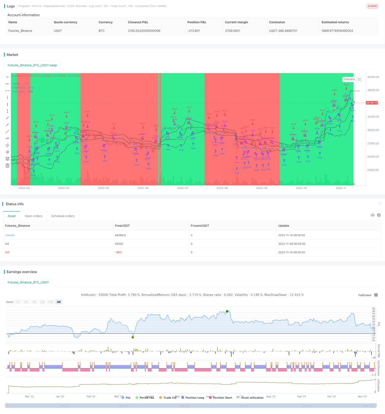
/*backtest
start: 2022-11-09 00:00:00
end: 2023-11-15 00:00:00
period: 1d
basePeriod: 1h
exchanges: [{"eid":"Futures_Binance","currency":"BTC_USDT"}]
*/


//@version=2
strategy("Noro's Bands Scalper Strategy v1.2", shorttitle = "Scalper str 1.2", overlay=true, default_qty_type = strategy.percent_of_equity, default_qty_value=100.0, pyramiding=0)
- 1