概述
本策略名称为“基于轨迹平均振幅的多时间帧交易策略”。它的主要思想是通过引入一个拟合价格轨迹的粒子,基于粒子与价格之间的平均振幅来构建交易信号。
策略原理
该策略首先定义了一个拟合价格轨迹的粒子。该粒子受引力和惯性的影响,其运动轨迹会围绕价格振荡。然后计算粒子与价格之间的平均偏离距离,并以此构建上下轨道。当价格突破上轨或下轨时,发出交易信号。
具体来说,策略中定义的粒子位置公式为:
pos:=if pos<close
     nz(pos[1])+grav+traj
else
     nz(pos[1])-(grav)+traj
这里grav代表引力项,使粒子向价格趋近;traj代表惯性项,使粒子保持运动趋势。这两个项结合使粒子围绕价格振荡。
然后计算价格与粒子之间的平均偏离距离avgdist,并以此构建上下轨道:
bbl=pos-sma(avgdist,varb)
bbh=pos+sma(avgdist,varb)
最后,当价格大于上轨时做多,小于下轨时做空。
策略优势
相比传统的移动平均线策略,本策略有以下优势:
- 利用粒子轨迹更好地模拟价格波动;
- 上下轨道可基于历史平均振幅自适应调整,有利于捕捉突破;
- 多时间框架设计,可以在高低时间框架之间切换,捕捉更多交易机会。
策略风险
本策略也存在一些风险:
- 粒子运动参数设置不当可能导致虚假信号或漏失信号;
- 多时间框架之间切换时可能出现信号冲突;
- 突破上下轨道信号可能会增加止损风险。
对应风险管理措施包括:优化参数以减少虚假信号,定义清晰的时间框架择时规则,设置适当的止损位置等。
策略优化方向
本策略可从以下几个方面进行优化:
- 优化粒子运动相关参数,拟合价格轨迹;
- 增加时间框架的层数,在更高级时间框架确认信号;
- 加入波动率指标判断,避免在市场剧烈波动时产生信号;
- 优化止损策略,降低单笔止损。
总结
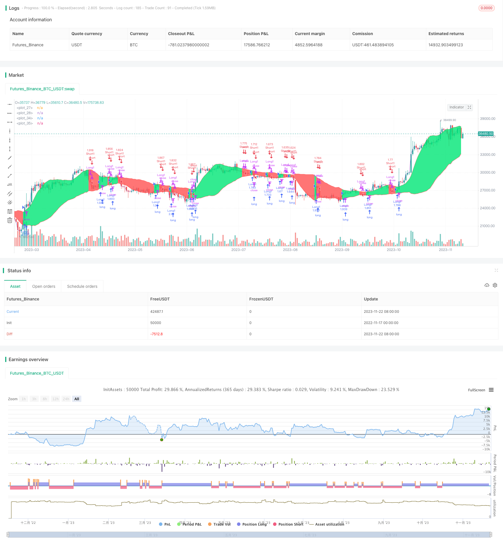
本策略通过引入价格轨迹拟合的方式改进了移动平均线策略,具有参数自适应、多时间框架、止损优化等特点。其关键在于找到合适的粒子运动方程来模拟价格。虽然仍需进一步测试和优化,但基本思路是可行的,值得进一步研究。
策略源码
/*backtest
start: 2022-11-17 00:00:00
end: 2023-11-23 00:00:00
period: 1d
basePeriod: 1h
exchanges: [{"eid":"Futures_Binance","currency":"BTC_USDT"}]
*/

//@version=4
//2 revert
strategy("Jomy's Gyroscopic Bands",precision=8,commission_value=.03,overlay=true,initial_capital =10000, default_qty_type=strategy.percent_of_equity, default_qty_value=100,  pyramiding=0)//,calc_on_order_fills= true, calc_on_every_tick=false)
leverage=input(1,"leverage")
a=0
a:= if volume > -1
    nz(a[1])+1
else
    nz(a)

vara=input(4.0,"variable a (10 to the power of __ ",step=.5)
vara:=pow(10,vara)
varb=input(12,"variable b")
pos=0.0
pos:=if a<=5
    close
else
    nz(pos[1])
grav=1/sqrt((close*close))*vara
traj=0.0
traj:=(nz(close[1])-nz(close[2])+nz(traj[1])*varb)/(varb+1)
pos:=if pos<close
    nz(pos[1])+grav+traj
else
    nz(pos[1])-(grav)+traj

plot(pos,color=color.white)
plot(close)

avgdist=abs(close-pos)
bbl=pos-sma(avgdist,varb)
bbh=pos+sma(avgdist,varb)

plbbh=plot(bbh,color=color.red)
plbbl=plot(bbl,color=color.red)

long = close>pos
short = close<pos

fill(plbbh,plbbl,color=long?color.lime:color.red)
//bgcolor(close>bbh?color.lime:close<bbl?color.red:na,transp=90)

strategy.entry("Long1",strategy.long,when=long,qty=(strategy.equity*leverage/open))
strategy.close("Long1",when=not long)
strategy.entry("Short1",strategy.short,when=short,qty=(strategy.equity*leverage/open))
strategy.close("Short1",when=not short)


//plot(strategy.equity,color=color.lime,linewidth=4)