The Smooth Moving Average Ribbon Strategy

Author: ChaoZhang, Date: 2023-12-11 14:48:35
Tags:

Overview

This strategy constructs a smooth price band using smooth moving averages and integrates various smooth moving averages to filter the trend in real time. It belongs to a typical trend following strategy.

Strategy Principle

Construct a smooth price band to track price changes using smooth moving averages.
The strategy supports various moving average types as the calculation method for smooth moving averages, such as EMA, SMMA, KAMA, etc.
It supports 1-5 layers of stacking smoothness on these moving averages to obtain an even smoother price band.
It also supports adding Bollinger Bands between prices and moving averages to better capture price changes.
By enabling an additional moving average filter, it can filter out fluctuations better and identify trend directions. The filter also supports multiple moving average types.
Combined with pattern recognition indicators, it can automatically identify buy and sell signals.

By constructing a smooth price band to capture price trends, and integrating a moving average filter to confirm trend directions, this strategy belongs to a typical trend following strategy. By adjusting parameters, it can be flexibly adapted to different products and timeframes.

Advantages

Constructing price bands can track price trend changes more smoothly, reducing the probability of missing opportunities.
Supporting multiple moving average types allows selecting suitable moving averages based on different timeframes and products, improving the adaptability of the strategy.
1-5 layers of stacking smoothness can significantly improve the tracking capability of price changes and capture trend reversal points more precisely.
The moving average filter can effectively reduce invalid signals and improve win rate.
By adjusting moving average lengths, it can be adapted to different timeframes. Multi-timeframe verification can further improve strategy performance.
Supporting black glass display enables clear and intuitive observation of price band trends.

Risks

Strong in tracking long-term trends, but poor in tracking and reacting to short-term fluctuations, tending to generate more invalid signals in range-bound markets.
In violent price surges and plunges, the lagging of smooth moving averages may miss the best entry timing.
Excessive stacking of moving averages may overly smooth price changes and cause inaccurate identifications of buy and sell points.
If the enabled moving average length parameters are improperly set, it may generate a large number of false signals.

Solutions:

Appropriately shorten moving average lengths to accelerate reaction to price changes.
Adjust stacking times to reduce over-smoothness.
Optimize and test moving average combinations to select optimal parameters.
Use multi-timeframe verification with other indicators to reduce false signals.

Optimization Directions

Test and optimize combinations of moving average types to select optimal parameters.
Test and optimize moving average length parameters to adapt to more products and timeframes.
Try different stacking smoothness times to find the optimal balance point.
Try adding Bollinger Bands as an auxiliary indicator.
Test different additional moving averages as filters.
Use multi-timeframe verification with other indicators.

Conclusion

This strategy belongs to a typical trend following strategy that continuously tracks price trends by constructing smooth moving average bands and avoids invalid signals with assisting filters. Its advantage lies in constructing smooth price bands to better capture turns in price trends. It also has certain risks of lagging. By parameter optimization and indicator optimization, the strategy performance can be continuously improved and is worth further research.

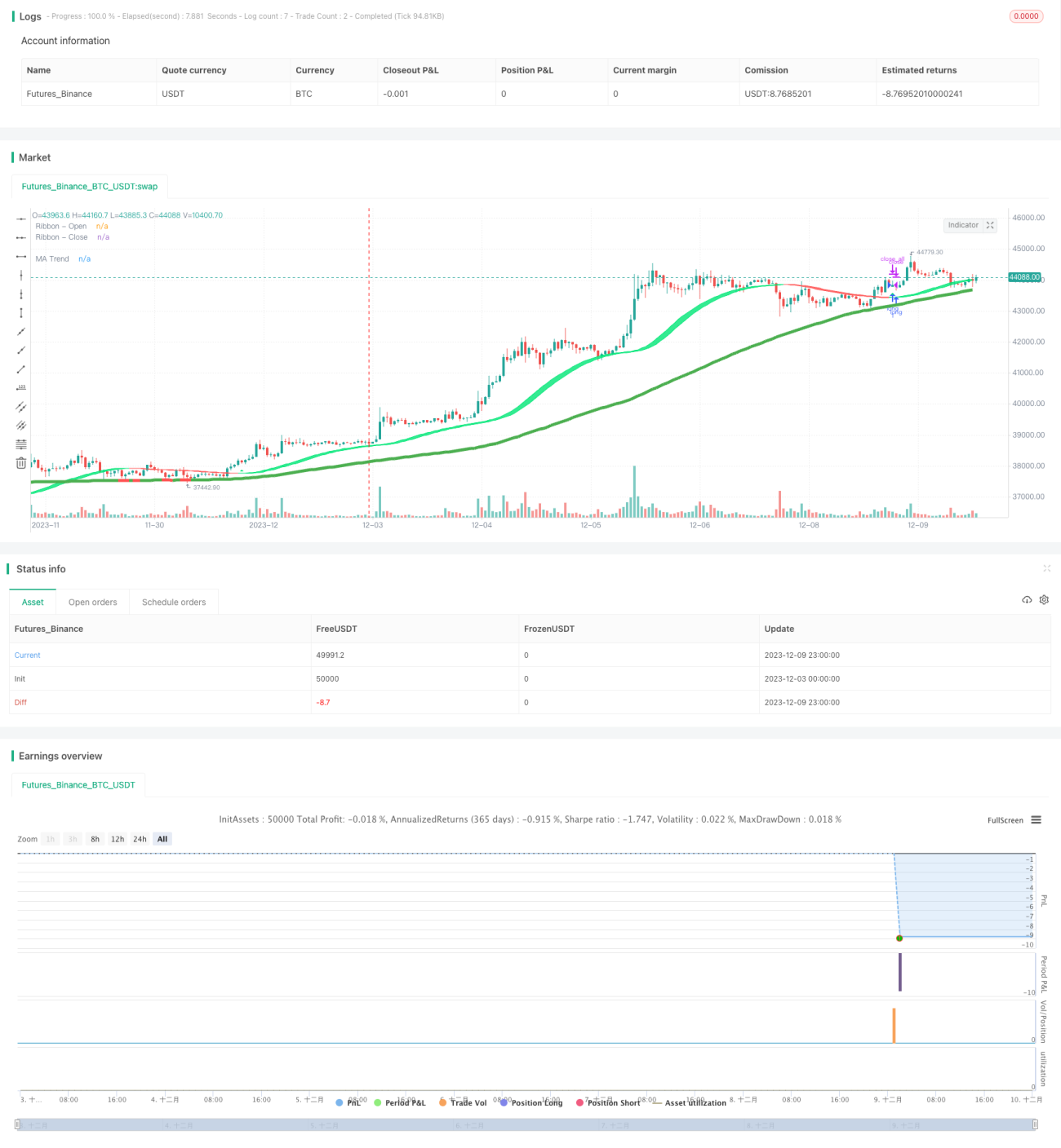
/*backtest
start: 2023-12-03 00:00:00
end: 2023-12-10 00:00:00
period: 1h
basePeriod: 15m
exchanges: [{"eid":"Futures_Binance","currency":"BTC_USDT"}]
*/

//@version=4
// Copyright (c) 2007-present Jurik Research and Consulting. All rights reserved.
// Copyright (c) 2018-present, Alex Orekhov (everget)
// Thanks to everget for code for more advanced moving averages
// Smooth Moving Average Ribbon [STRATEGY] @PuppyTherapy script may be freely distributed under the MIT license.
strategy( title="Smooth Moving Average Ribbon [STRATEGY] @PuppyTherapy", overlay=true )

// ---- CONSTANTS ----
lsmaOffset = 1
almaOffset = 0.85
almaSigma  = 6
phase = 2
power = 2

// ---- GLOBAL FUNCTIONS ----
kama(src, len)=>
    xvnoise = abs(src - src[1])
    nfastend = 0.666
    nslowend = 0.0645
    nsignal = abs(src - src[len])
    nnoise = sum(xvnoise, len)
    nefratio = iff(nnoise != 0, nsignal / nnoise, 0)
    nsmooth = pow(nefratio * (nfastend - nslowend) + nslowend, 2)
    nAMA = 0.0
    nAMA := nz(nAMA[1]) + nsmooth * (src - nz(nAMA[1]))

t3(src, len)=>
    xe1_1 = ema(src,    len)
    xe2_1 = ema(xe1_1,  len)
    xe3_1 = ema(xe2_1,  len)
    xe4_1 = ema(xe3_1,  len)
    xe5_1 = ema(xe4_1,  len)
    xe6_1 = ema(xe5_1,  len)
    b_1 = 0.7
    c1_1 = -b_1*b_1*b_1
    c2_1 = 3*b_1*b_1+3*b_1*b_1*b_1
    c3_1 = -6*b_1*b_1-3*b_1-3*b_1*b_1*b_1
    c4_1 = 1+3*b_1+b_1*b_1*b_1+3*b_1*b_1
    nT3Average_1 = c1_1 * xe6_1 + c2_1 * xe5_1 + c3_1 * xe4_1 + c4_1 * xe3_1
    
// The general form of the weights of the (2m + 1)-term Henderson Weighted Moving Average
getWeight(m, j) =>
    numerator = 315 * (pow(m + 1, 2) - pow(j, 2)) * (pow(m + 2, 2) - pow(j, 2)) * (pow(m + 3, 2) - pow(j, 2)) * (3 * pow(m + 2, 2) - 11 * pow(j, 2) - 16)
    denominator = 8 * (m + 2) * (pow(m + 2, 2) - 1) * (4 * pow(m + 2, 2) - 1) * (4 * pow(m + 2, 2) - 9) * (4 * pow(m + 2, 2) - 25)

    denominator != 0
         ? numerator / denominator
         : 0

hwma(src, termsNumber) =>
    sum = 0.0
    weightSum = 0.0
    
    termMult = (termsNumber - 1) / 2

    for i = 0 to termsNumber - 1
        weight = getWeight(termMult, i - termMult)
        sum := sum + nz(src[i]) * weight
        weightSum := weightSum + weight

    sum / weightSum

get_jurik(length, phase, power, src)=>
    phaseRatio = phase < -100 ? 0.5 : phase > 100 ? 2.5 : phase / 100 + 1.5
    beta = 0.45 * (length - 1) / (0.45 * (length - 1) + 2)
    alpha = pow(beta, power)
    jma = 0.0
    e0 = 0.0
    e0 := (1 - alpha) * src + alpha * nz(e0[1])
    e1 = 0.0
    e1 := (src - e0) * (1 - beta) + beta * nz(e1[1])
    e2 = 0.0
    e2 := (e0 + phaseRatio * e1 - nz(jma[1])) * pow(1 - alpha, 2) + pow(alpha, 2) * nz(e2[1])
    jma := e2 + nz(jma[1])

variant(src, type, len ) =>
    v1 = sma(src, len)                                                  // Simple
    v2 = ema(src, len)                                                  // Exponential
    v3 = 2 * v2 - ema(v2, len)                                          // Double Exponential
    v4 = 3 * (v2 - ema(v2, len)) + ema(ema(v2, len), len)               // Triple Exponential
    v5 = wma(src, len)                                                  // Weighted
    v6 = vwma(src, len)                                                 // Volume Weighted
    v7 = na(v5[1]) ? sma(src, len) : (v5[1] * (len - 1) + src) / len    // Smoothed
    v8 = wma(2 * wma(src, len / 2) - wma(src, len), round(sqrt(len)))   // Hull
    v9 = linreg(src, len, lsmaOffset)                                   // Least Squares
    v10 = alma(src, len, almaOffset, almaSigma)                         // Arnaud Legoux
    v11 = kama(src, len)                                                // KAMA
    ema1 = ema(src, len)
    ema2 = ema(ema1, len)
    v13 = t3(src, len)                                                  // T3
    v14 = ema1+(ema1-ema2)                                              // Zero Lag Exponential
    v15 = hwma(src, len)                                                // Henderson Moving average thanks to  @everget
    ahma = 0.0
    ahma := nz(ahma[1]) + (src - (nz(ahma[1]) + nz(ahma[len])) / 2) / len //Ahrens Moving Average 
    v16 = ahma
    v17 = get_jurik( len, phase, power, src) 
    type=="EMA"?v2 : type=="DEMA"?v3 : type=="TEMA"?v4 : type=="WMA"?v5 : type=="VWMA"?v6 :
     type=="SMMA"?v7 : type=="Hull"?v8 : type=="LSMA"?v9 : type=="ALMA"?v10 : type=="KAMA"?v11 :
     type=="T3"?v13 : type=="ZEMA"?v14 : type=="HWMA"?v15 : type=="AHMA"?v16 : type=="JURIK"?v17 : v1

smoothMA(o, h, l, c, maLoop, type, len) =>
	ma_o = 0.0
	ma_h = 0.0
	ma_l = 0.0
	ma_c = 0.0
	if maLoop == 1
		ma_o := variant(o, type, len)
		ma_h := variant(h, type, len)
		ma_l := variant(l, type, len)
		ma_c := variant(c, type, len)
	if maLoop == 2
		ma_o := variant(variant(o ,type, len),type, len)
		ma_h := variant(variant(h ,type, len),type, len)
		ma_l := variant(variant(l ,type, len),type, len)
		ma_c := variant(variant(c ,type, len),type, len)
	if maLoop == 3
		ma_o := variant(variant(variant(o ,type, len),type, len),type, len)
		ma_h := variant(variant(variant(h ,type, len),type, len),type, len)
		ma_l := variant(variant(variant(l ,type, len),type, len),type, len)
		ma_c := variant(variant(variant(c ,type, len),type, len),type, len)
	if maLoop == 4
		ma_o := variant(variant(variant(variant(o ,type, len),type, len),type, len),type, len)
		ma_h := variant(variant(variant(variant(h ,type, len),type, len),type, len),type, len)
		ma_l := variant(variant(variant(variant(l ,type, len),type, len),type, len),type, len)
		ma_c := variant(variant(variant(variant(c ,type, len),type, len),type, len),type, len)
	if maLoop == 5
		ma_o := variant(variant(variant(variant(variant(o ,type, len),type, len),type, len),type, len),type, len)
		ma_h := variant(variant(variant(variant(variant(h ,type, len),type, len),type, len),type, len),type, len)
		ma_l := variant(variant(variant(variant(variant(l ,type, len),type, len),type, len),type, len),type, len)
		ma_c := variant(variant(variant(variant(variant(c ,type, len),type, len),type, len),type, len),type, len)
    [ma_o, ma_h, ma_l, ma_c]

smoothHA( o, h, l, c ) =>
    hao = 0.0
    hac = ( o + h + l + c ) / 4
    hao := na(hao[1])?(o + c / 2 ):(hao[1] + hac[1])/2
    hah = max(h, max(hao, hac))
    hal = min(l, min(hao, hac))
	[hao, hah, hal, hac]

// ---- Main Ribbon ----
haSmooth   = input(true, title=" Use HA as source ? " )
length     = input(11, title=" MA1 Length", minval=1, maxval=1000)
maLoop     = input(3, title=" Nr. of MA1 Smoothings ", minval=1, maxval=5)
type       = input("EMA", title="MA Type", options=["SMA", "EMA", "DEMA", "TEMA", "WMA", "VWMA", "SMMA", "Hull", "LSMA", "ALMA", "KAMA", "ZEMA", "HWMA", "AHMA", "JURIK", "T3"])
haSmooth2  = input(true, title=" Use HA as source ? " )

// ---- Trend ----
ma_use    = input(true, title=" ----- Use MA Filter ( For Lower Timeframe Swings / Scalps ) ? ----- " )
ma_source = input(defval = close, title = "MA - Source", type = input.source)
ma_length = input(100,title="MA - Length", minval=1 )
ma_type   = input("SMA", title="MA - Type", options=["SMA", "EMA", "DEMA", "TEMA", "WMA", "VWMA", "SMMA", "Hull", "LSMA", "ALMA", "KAMA", "ZEMA", "HWMA", "AHMA", "JURIK", "T3"])
ma_useHA  = input(defval = false, title = "Use HA Candles as Source ?")
ma_rsl    = input(true, title = "Use Rising / Falling Logic ?" )

// ---- BODY SCRIPT ----
[ ha_open, ha_high, ha_low, ha_close ] = smoothHA(open, high, low, close)

_open_ma  = haSmooth ? ha_open : open
_high_ma  = haSmooth ? ha_high : high
_low_ma   = haSmooth ? ha_low : low
_close_ma = haSmooth ? ha_close : close

[ _open, _high, _low, _close ] = smoothMA( _open_ma, _high_ma, _low_ma, _close_ma, maLoop, type, length)
[ ha_open2, ha_high2, ha_low2, ha_close2 ] = smoothHA(_open, _high, _low, _close)

_open_ma2  = haSmooth2 ? ha_open2 : _open
_high_ma2  = haSmooth2 ? ha_high2 : _high
_low_ma2   = haSmooth2 ? ha_low2 : _low
_close_ma2 = haSmooth2 ? ha_close2 : _close

ribbonColor = _close_ma2 > _open_ma2 ? color.lime : color.red
p_open  = plot(_open_ma2,  title="Ribbon - Open",   color=ribbonColor, transp=70)
p_close = plot(_close_ma2, title="Ribbon - Close",  color=ribbonColor, transp=70)
fill(p_open, p_close, color = ribbonColor, transp = 40 )

// ----- FILTER

ma = 0.0
if ma_use == true
    ma := variant( ma_useHA ? ha_close : ma_source, ma_type,  ma_length )

maFilterShort = ma_use ? ma_rsl ? falling(ma,1) : ma_useHA ? ha_close : close < ma : true 
maFilterLong  = ma_use ? ma_rsl ? rising(ma,1) : ma_useHA ? ha_close : close > ma : true 


colorTrend = rising(ma,1) ? color.green : color.red
plot( ma_use ? ma : na, title="MA Trend",  color=colorTrend, transp=80, transp=70, linewidth = 5)

long     = crossover(_close_ma2, _open_ma2 ) and maFilterLong
short    = crossunder(_close_ma2, _open_ma2 ) and maFilterShort
closeAll = cross(_close_ma2, _open_ma2 )

plotshape( short , title="Short", color=color.red,  transp=80, style=shape.triangledown, location=location.abovebar, size=size.small)
plotshape( long ,  title="Long",  color=color.lime, transp=80, style=shape.triangleup,   location=location.belowbar, size=size.small)

//* Backtesting Period Selector | Component *//
//* Source: https://www.tradingview.com/script/eCC1cvxQ-Backtesting-Period-Selector-Component *//
testStartYear   = input(2018, "Backtest Start Year",minval=1980)
testStartMonth  = input(1, "Backtest Start Month",minval=1,maxval=12)
testStartDay    = input(1, "Backtest Start Day",minval=1,maxval=31)
testPeriodStart = timestamp(testStartYear,testStartMonth,testStartDay,0,0)
testStopYear    = 9999 //input(9999, "Backtest Stop Year",minval=1980)
testStopMonth   = 12 // input(12, "Backtest Stop Month",minval=1,maxval=12)
testStopDay     = 31 //input(31, "Backtest Stop Day",minval=1,maxval=31)
testPeriodStop  = timestamp(testStopYear,testStopMonth,testStopDay,0,0)
testPeriod() => time >= testPeriodStart and time <= testPeriodStop ? true : false

if testPeriod() and long
    strategy.entry( "long", strategy.long )

if testPeriod() and short
    strategy.entry( "short", strategy.short )
    
if closeAll
    strategy.close_all( when = closeAll )

More

Forums
|
API
|
Github
|
About
|
SiteMap