Laguerre RSI Trading Strategy

Overview
The Laguerre RSI trading strategy is based on John EHLERS’ Laguerre filter applied to the RSI indicator. By adjusting the α coefficient, this strategy increases or decreases the lag and smoothness of the RSI to filter out noise and generate clearer trading signals.
Strategy Logic
The core indicator of this strategy is Laguerre RSI. Its calculation formula is as follows:
L0 = (1-γ)Src + γL0[1]
L1 = -γL0 + L0[1] + γL1[1]
L2 = -γL1 + L1[1] + γL2[1]
L3 = -γL2 + L2[1] + γL3[1]
Here γ=1-α, α is an adjustable coefficient, Src represents price. L0 to L3 are 4 indicators containing recursive relationships. On this basis, the current up integral cu and down integral cd can be calculated:
cu = (L0>L1 ? L0-L1 : 0) + (L1>L2 ? L1-L2 : 0) + (L2>L3 ? L2-L3 : 0)
cd = (L0<L1 ? L1-L0 : 0) + (L1<L2 ? L2-L1 : 0) + (L2<L3 ? L3-L2 : 0)
Then Laguerre RSI can be calculated using cu and cd:
LaRSI = cu / (cu + cd)
Through the recursive filter structure, Laguerre RSI retains the trend identification capability of RSI while filtering out a lot of random noise, generating clearer and smoother trading signals.
The specific trading rules are:
Go long when Laguerre RSI crosses above 20, and go short when Laguerre RSI crosses below 80.
Advantage Analysis
The main advantages of Laguerre RSI strategy are:
-
Effectively filter the noise of RSI through Laguerre filter structure, making trading signals clearer and more reliable
-
The adjustable α coefficient makes the strategy parameters flexible for optimization to adapt to more market environments
-
Retains the long-term validity of RSI while enabling momentum identification through filtering, integrating trend and overbought/oversold
-
Simple and intuitive strategy rules that are easy to implement and perform well in various market environments
Risk Analysis
The main risks of this strategy are:
-
Improper settings of α may lead to excessive lag or over-filtering, thus missing price changes
-
Frequent trading losses may occur in volatile markets
-
Some upside opportunities may be missed in long-term sustained bull markets
Optimization Directions
This strategy can be optimized from the following aspects:
-
Use machine learning algorithms to optimize the α coefficient setting
-
Add stop loss mechanisms to reduce loss risk
-
Combine other indicators to filter false signals
-
Increase the quantitative easing model to lock in profits at specific stages
Conclusion
The Laguerre RSI strategy effectively identifies overbought and oversold situations through filtering mechanisms while avoiding interference from noise when issuing trading signals. This simple and practical strategy has large optimization space for parameters and can adapt to various market environments. It is a recommended trading strategy.
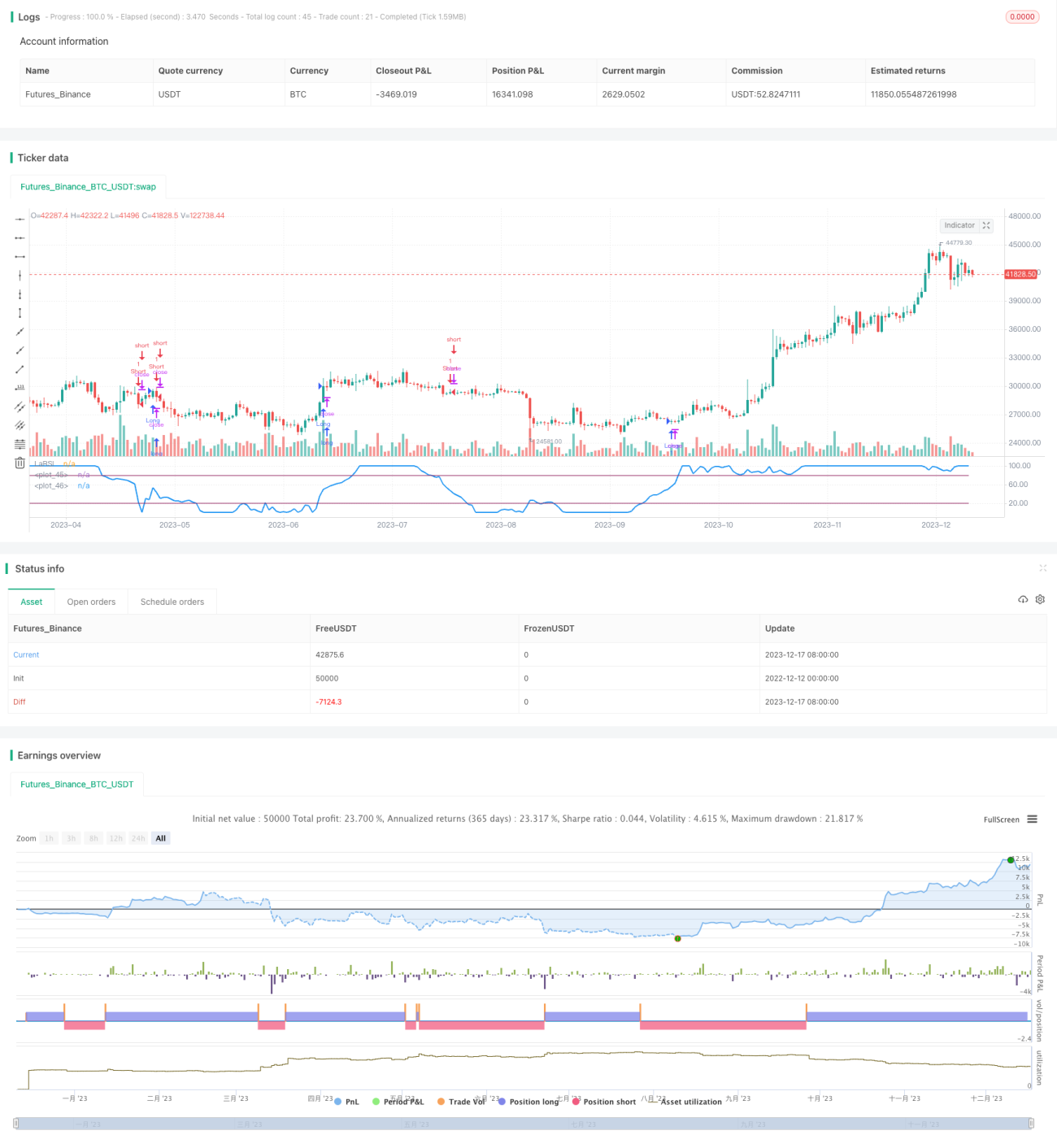
/*backtest
start: 2022-12-12 00:00:00
end: 2023-12-18 00:00:00
period: 1d
basePeriod: 1h
exchanges: [{"eid":"Futures_Binance","currency":"BTC_USDT"}]
*/

// This source code is subject to the terms of the Mozilla Public License 2.0 at https://mozilla.org/MPL/2.0/
// © mertriver1
// Developer: John EHLERS
//@version=3- 1