概述
自适应趋势跟随策略是一种结合布林带指标和均线指标,动态调整趋势强度因子,实现趋势跟随和止损的量化交易策略。该策略运用布林带指标计算价格波动率,据此动态计算合理的趋势强度,然后结合ATR指标绘制自适应的趋势通道,实现对牛熊趋势的判断和跟随。同时,策略内置止损机制,可以有效控制风险。
策略原理
该策略的核心指标是布林带。布林带是由中轨、上轨和下轨组成。中轨为n日的简单移动平均线,上轨是中轨+k倍的n日标准差,下轨是中轨-k倍的n日标准差。这里选取20日中轨和2倍标准差构建布林带。
然后计算布林带的带宽(上轨-下轨)与中轨的比值,称为“强度因子”。该比值反映了当前市场波动率和趋势强度。我们设定强度因子的最大最小值,防止其过大或过小。
得到合理的强度因子后,结合ATR指标,上下轨分别向上和向下移动ATR*强度因子这个距离,形成自适应的趋势通道。当收盘价由下向上突破上轨时,做多;由上向下突破下轨时,做空。
此外,策略还设置止损机制。当多头仓位形成后,若价格跌破开仓时的最低点,则止损平仓;空头仓位亦然。
策略优势
该策略具有以下优势:
自适应性强。强度因子的计算方式使得策略可以根据市场波动率动态调整通道宽度,在趋势牛市中通道加宽,在震荡市中通道收窄,实现对不同类型市场的自适应。
操作频率适中。相比简单移动平均线策略,布林带策略调整通道的频率更低,避免了不必要的频繁开平仓。
入场准确。突破上下轨这一入场方式可以有效过滤市场噪音,确保以高概率捕捉到趋势的开启。
有止损机制。内置的止损方式可以有效控制单笔亏损,是该策略的一大优势。
策略风险
该策略也存在一些风险:
参数敏感性较大。布林带的周期n和倍数k对结果影响很大,需要反复测试找到最佳参数组合。
布林带轨道发散时无法跟踪趋势。当价格出现剧烈波动时,布林带轨道会快速拉开,导致无法跟踪趋势。这时需要暂停策略,等待轨道收敛后再运行。
有时会产生错误信号。布林带策略并非完美,也会有一定的错误信号产生,这需要承担相应的亏损。
止损方式较为简单。该策略的止损只考虑开仓后最高价和最低价,没有结合波动率等更复杂的止损方式,可能会过于激进或者保守,需要优化。
策略优化方向
该策略还需要从以下几个方面进行优化:
测试不同币种和不同周期参数的效果。策略的参数可以针对不同币种和周期进行优化,提高策略适应性。
优化止损机制。可以引入移动止损、振荡止损、追踪止损等,使止损方式更加智能化。
结合其他指标过滤进场。可以加入如MACD、KDJ等指标,避免布林带在横盘震荡市产生错误信号。
增加仓位管理机制。实现追踪止盈、金字塔加仓、固定比例仓位等管理方式,可以提高策略收益率。
进行回测优化。通过扩大回测时间范围、调整参数、分析回测报告等,全面检查策略效果,找到最优参数。
总结
自适应趋势跟随策略整体来说是一种较为成熟的量化策略。它运用布林带指标动态捕捉趋势,配合ATR指标构建自适应通道,实现对多空趋势的判断。同时内置止损机制控制风险。该策略优势在于操作频率适中、入场准确、风险控制性较好。但也存在一些问题,需要从参数选择、止损方式、信号过滤等方面进行优化,使策略更加稳健和智能化。
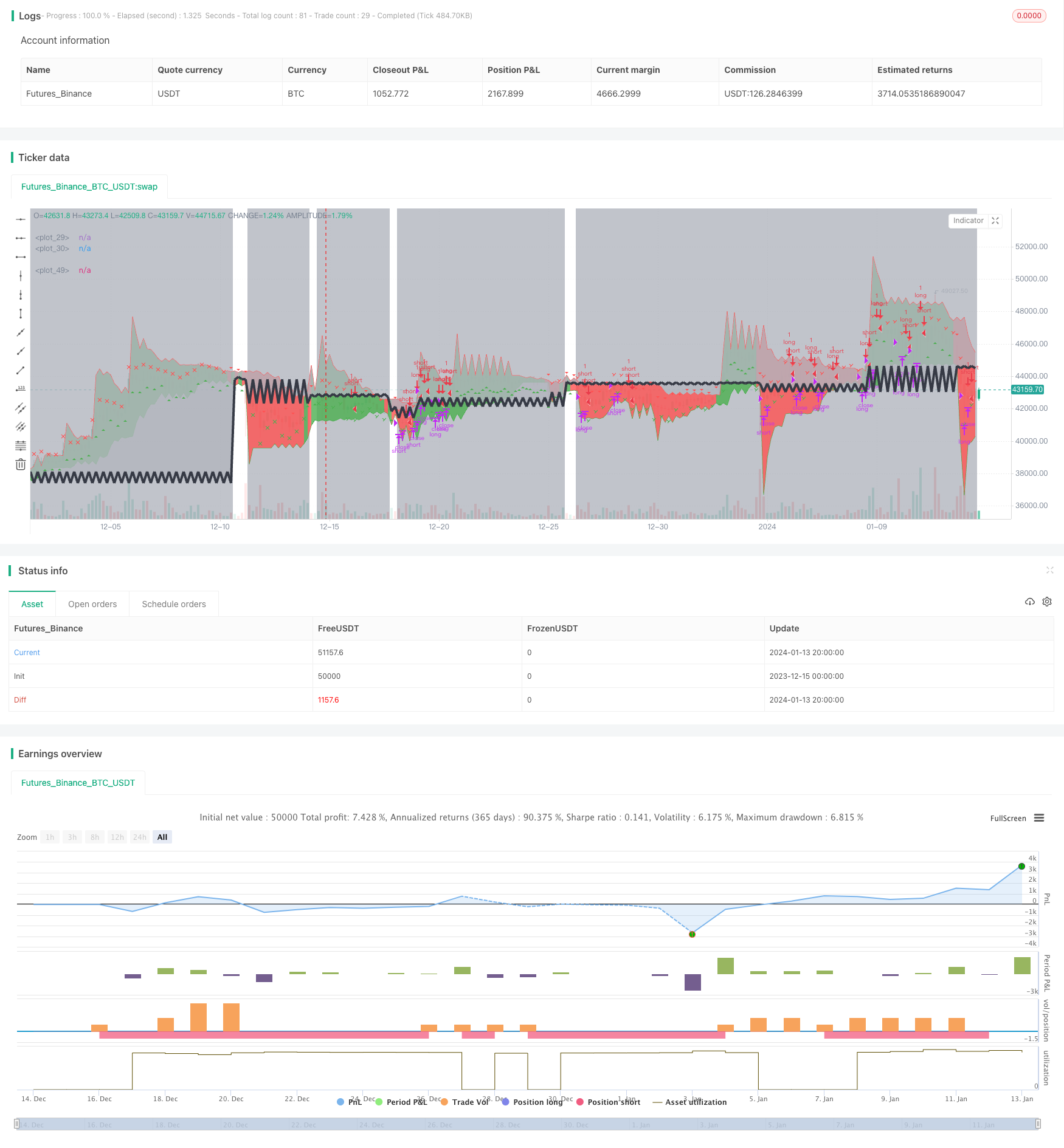
/*backtest
start: 2023-12-15 00:00:00
end: 2024-01-14 00:00:00
period: 4h
basePeriod: 15m
exchanges: [{"eid":"Futures_Binance","currency":"BTC_USDT"}]
*/

//@version=2
strategy("[Th] Adaptive Trend v1", shorttitle="[TH] Adaptive Trend", overlay=true)

Pd=input(2, minval=1,maxval = 100, title="Period")
Bw=input(50, minval=1,maxval = 100, title="Bandwidth")
minFactor = input(0.5, minval=0.1, maxval=1.0, step=0.1, title="Minimum Factor")
maxFactor = input(3.00, minval=0.2, maxval=5.0, step=0.1, title="Maximum Factor")
plot_trend=input(true, title="Plot trend")

plot_losscut = input(true, title="Plot losscut")

/////////////// Calculate the BB's ///////////////
basisBB = ema(close, 20)
devBB     = 2 * stdev(close, 20)
upperBB = basisBB + devBB
lowerBB = basisBB - devBB
//plot(upperBB)
//plot(lowerBB)

///////////// Trend ////////////////////////////

rawFactor = ((upperBB-lowerBB)/basisBB)*Bw
Factor = rawFactor > minFactor ? (rawFactor > maxFactor ? maxFactor : rawFactor) : minFactor

Up=hl2-(Factor*atr(Pd))
Dn=hl2+(Factor*atr(Pd))
TrendUp=close[1]>TrendUp[1]? max(Up,TrendUp[1]) : Up
TrendDown=close[1]<TrendDown[1]? min(Dn,TrendDown[1]) : Dn
TrendUpPlot=plot(plot_trend?TrendUp:na, style=line, color=green, linewidth=1)
TrendDownPlot=plot(plot_trend?TrendDown:na, style=line, color=red, linewidth=1)
Trend = close > TrendDown[1] ? 1: close< TrendUp[1]? -1: nz(Trend[1],1)
fill(TrendUpPlot,TrendDownPlot, color=Trend == 1 ? green : red, transp=80)
sig_trend_long = Trend[1] == -1 and Trend == 1
sig_trend_short = Trend[1] == 1 and Trend == -1

///////////// Loss Cut ////////////////////////////
price_cut = sig_trend_long[1] or sig_trend_short[1] or sig_reentry_long[1] or sig_reentry_short[1] ? open : price_cut[1]
current_trend = sig_trend_long[1] ? 1 : (sig_trend_short[1] ? -1 : current_trend[1])

sig_loss_cut = sig_trend_long or sig_trend_short ? false : ( current_trend == 1 ? (price_cut > low) : (current_trend == -1 ? (price_cut < high) : false) )
has_position = sig_loss_cut ? false : ((sig_trend_long[1] or sig_trend_short[1] or sig_reentry_long[1] or sig_reentry_short[1]) ? true : has_position[1])
sig_reentry_long = not has_position and current_trend == 1 and low > price_cut
sig_reentry_short = not has_position and current_trend == -1 and high < price_cut

bgcolor(plot_losscut and ( not has_position or sig_loss_cut ) ? silver : white, transp=70)
plotshape(plot_losscut and sig_loss_cut and current_trend == 1? 1 : na, color=green, style=shape.xcross, location=location.belowbar ,size=size.tiny)
plotshape(plot_losscut and sig_loss_cut and current_trend == -1? 1 : na, color=red, style=shape.xcross, location=location.abovebar ,size=size.tiny)

LossCutPlot = plot(plot_losscut ? price_cut : na, linewidth=4, color=black, transp=60)
fill(TrendDownPlot, LossCutPlot, color=silver, transp=90)

plotshape(sig_trend_long or sig_reentry_long ? Trend : na, title="Up Entry Arrow", color=green, style=shape.triangleup, location=location.belowbar, size=size.tiny)
plotshape(sig_trend_short or sig_reentry_short ? Trend : na, title="Down Entry Arrow",color=red, style=shape.triangledown, size=size.tiny)


///////////// Strategy ////////////////////////////
if true

    strategy.entry('long', long=strategy.long, comment='Long', when=sig_trend_long or sig_reentry_long)
    strategy.entry('short', long=strategy.short, comment='Short', when=sig_trend_short or sig_reentry_short)

    if(current_trend == 1)
        strategy.close('long', when=sig_loss_cut == true)
        //strategy.exit('lc',from_entry='long', stop=price_cut)

    if( current_trend == -1 )
        strategy.close('short', when=sig_loss_cut == true)
        //strategy.exit('sc',from_entry='short', stop=price_cut)