概述
该策略基于日线级别的海龚阿希K线,结合不同周期层面的动能分析,动态确定当前股价背后的支撑力量,从而判断建仓和平仓的时机。
策略原理
计算不同周期层面海龚阿希K线的收盘价。这是后续动能计算的基础。
分别计算月线和日线的开盘价与不同历史周期收盘价的涨跌幅。这反映了当前股价相对历史价格的动能强度。
对月线和日线的动能涨跌幅分别取平均,过滤掉部分噪音,得到稳定的月线、日线动能指标。
根据平均动能涨跌幅,可以计算得出当前股价能反映的市场支撑力量,即去除市场波动影响的价格。该价格可以看作当前真实股价的动能门槛。
当收盘价高于动能门槛时,进行逐月做多建仓。当收盘价低于动能门槛时,平仓止损。
优势分析
该策略最大的优势在于,它没有简单追随股价,而是基于股价背后的动能计算真实支撑力量,从而进行建仓和止损。这可以有效过滤震荡行情的噪音,锁定稳定上涨的机会。
另外,策略所基于的数据全部来自海龚阿希K线。这种特殊K线本身就可以减少过度依赖联结周期的问题。所以策略的稳定性会比其他K线策略更好。
风险分析
该策略最大的风险在于,动能计算都是基于历史价格。如果公司基本面和行情发生重大变化,历史价格的代表性就会下降,从而导致建仓和止损判断出现偏差。
此外,策略使用的是月度和日度周期。这意味着策略的实时性不高,无法对行情的急剧变化做出快速反应。这在行情突变时会带来止损风险。
为降低这些风险,可以考虑引入更高频的数据,以及公司基本面的实时反馈。或者结合其他更为主观的交易信号进行验收和优化。
优化方向
可以从以下几个方面继续优化该策略:
海龚阿希K线本身也可以进一步优化,如调整权重配置等。
增加更多不同周期的数据,构建出指数平均的动能评分机制,提高稳定性。
引入更高频如日内分钟线数据,以提高策略的实时性。
结合业绩预告、重组传闻等信息,对动能计算加入公司基本面的反馈。
可以考虑在月度建仓的基础上,增加日度或周度的止盈和加仓机制。
总结
该策略整体来说非常稳定,通过动能追踪的方式有效控制了风险。它最大的优势在于利用股价背后的动能力量判定真实行情,而不是单纯追随股价本身。下一步通过引入更多频率更高、信息更丰富的数据,有望进一步优化该策略,使其能更好地把握市场机会。
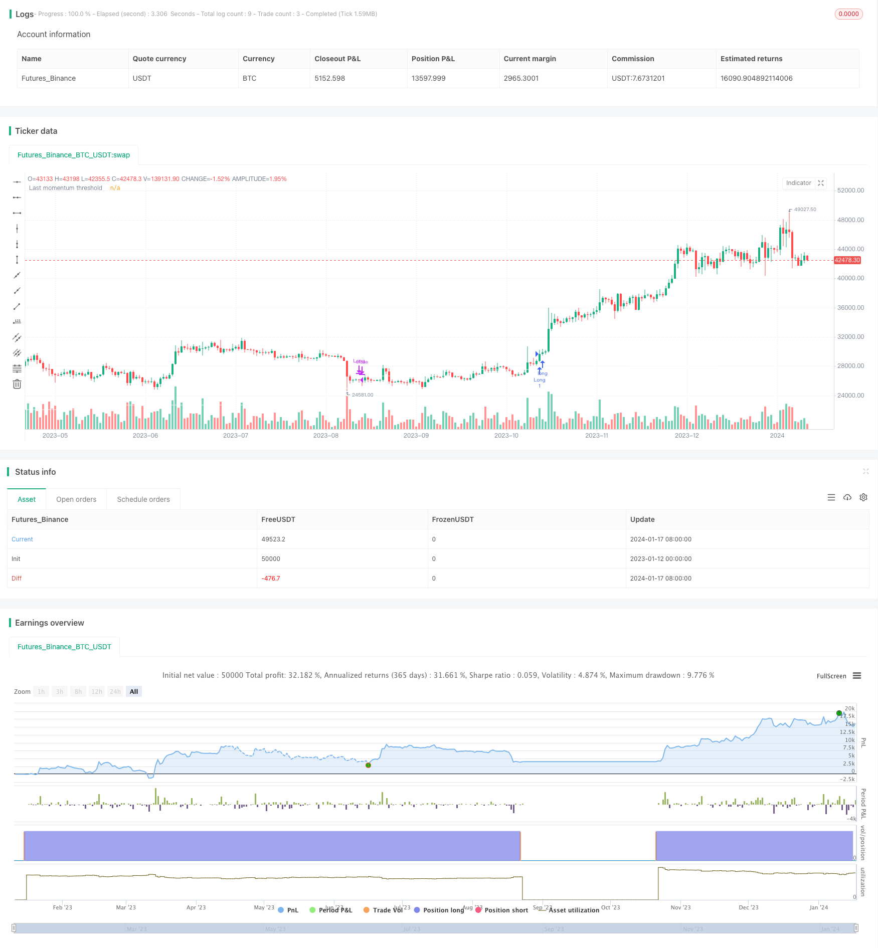
/*backtest
start: 2023-01-12 00:00:00
end: 2024-01-18 00:00:00
period: 1d
basePeriod: 1h
exchanges: [{"eid":"Futures_Binance","currency":"BTC_USDT"}]
*/

// This Pine Script™ code is subject to the terms of the Mozilla Public License 2.0 at https://mozilla.org/MPL/2.0/
// © FrancoPassuello

//@version=5
strategy("Heiken Ashi ADM", overlay=true)
haClose = (open + high + low + close) / 4
// prevHaOpen = line.new(na, na, na, na, width = 1)
haOpen = (open[1] + close[1]) / 2
// line.set_xy1(prevHaOpen, bar_index[1], nz(haOpen[1]))
// line.set_xy2(prevHaOpen, bar_index, haClose[1])


[monopen, _1monopen, _2monopen, _3monopen, _4monopen, _5monopen, _6monopen] = request.security(syminfo.tickerid, "M", [haOpen, haOpen[1], haOpen[2], haOpen[3], haOpen[4], haOpen[5], haOpen[6]] , barmerge.gaps_off, barmerge.lookahead_on)
[monclose, _1monclose, _3monclose, _6monclose] = request.security(syminfo.tickerid, "M", [haClose, haClose[1], haClose[3], haClose[6]] , barmerge.gaps_off, barmerge.lookahead_on)
[dayclose1, _21dayclose, _63dayclose, _126dayclose, dayclose] = request.security(syminfo.tickerid, "1D", [haClose[1], haClose[21], haClose[63], haClose[126], haClose], barmerge.gaps_off, barmerge.lookahead_on)
[dayopen1, _21dayopen, _63dayopen, _126dayopen] = request.security(syminfo.tickerid, "1D", [haOpen[1], haOpen[21], haOpen[63], haOpen[126]], barmerge.gaps_off, barmerge.lookahead_on)


get_rate_of_return(price1, price2) =>
    return_ = (price1/price2 -1)*100
    return_

m0 = get_rate_of_return(monclose, monopen)
m1 = get_rate_of_return(_1monclose, _1monopen)
m2 = get_rate_of_return(monclose, _2monopen)
m3 = get_rate_of_return(_1monclose, _3monopen)
m4 = get_rate_of_return(monclose, _4monopen)
m5 = get_rate_of_return(monclose, _5monopen)
m6 = get_rate_of_return(_1monclose, _6monopen)
MS = (m1 + m3 + m6)/100
CS = (m0 + m2 + m5)/100

d1 = get_rate_of_return(dayclose1, _21dayopen)
d2 = get_rate_of_return(dayclose1, _63dayopen)
d3 = get_rate_of_return(dayclose1, _126dayopen)
DS = (d1 + d2 + d3)/100

//Last (DAILY)
lastd_s_avg1 = DS/3

lastd_Approximate1 = dayclose1*(1-lastd_s_avg1)

last_approx1_d21 = lastd_Approximate1 / _21dayopen-1
last_approx1_d63 = lastd_Approximate1 / _63dayopen-1
last_approx1_d126 = lastd_Approximate1 / _126dayopen-1

lastd_s_avg2 = (last_approx1_d21 + last_approx1_d63 + last_approx1_d126) / 3
lastd_approximate2 = (dayclose1)*(1-(lastd_s_avg1 + lastd_s_avg2))
lastd_price = lastd_approximate2

//plot(lastd_price,color = color.rgb(255, 255, 255, 14), title = "Last momentum threshold")

//Last

last_s_avg1 = MS/3

last_Approximate1 = _1monclose*(1-last_s_avg1)

last_approx1_m1 = last_Approximate1 / _1monopen-1
last_approx1_m3 = last_Approximate1 / _3monopen-1
last_approx1_m6 = last_Approximate1 / _6monopen-1

last_s_avg2 = (last_approx1_m1 + last_approx1_m3 + last_approx1_m6) / 3
last_approximate2 = (_1monclose)*(1-(last_s_avg1 + last_s_avg2))
last_price = last_approximate2
Scoring_price = _1monclose*(1-CS)

plot(last_price,color = color.rgb(255, 255, 255, 14), title = "Last momentum threshold")
//plot(Scoring_price,color = color.rgb(234, 0, 255, 14), title = "Last momentum threshold")

//Long based on month close and being the first trade of the month.

var int lastClosedMonth = -1
limit_longCondition = _1monclose > last_approximate2 and (lastClosedMonth == -1 or month(time) != lastClosedMonth)

// Long based on day close and being the first trade of the month.
limit_Dlongcondition = dayclose1 > lastd_approximate2 and (lastClosedMonth == -1 or month(time) != lastClosedMonth)

// Close trade based on day close

DCloseLongCondition = dayclose1<lastd_approximate2

//Old standard Trading rules
longCondition = _1monclose > Scoring_price
MCloseLongCondition = _1monclose<Scoring_price
shortCondition = CS < 0

if (longCondition)
    strategy.entry("Long", strategy.long)


if (strategy.position_size > 0 and MCloseLongCondition)
    strategy.close("Long")
    lastClosedMonth := month(time)