概述
该策略运用多周期自适应移动平均线和折线风险评价指标,结合市场运行中的分型点进行走势预测与交易信号输出。策略名称为“多周期自适应走势预测策略”。
策略原理
策略的核心逻辑是分为两条主线。第一条主线是利用不同参数的自适应移动平均线nAMA构建多周期过滤判断系统,第二条主线是利用不同参数的折线风险评价系统out构建多周期风险评价体系。最后将两条主线进行组合,当短周期线超过长周期线时产生买入信号。当短周期线低于长周期线时产生卖出信号。
具体来说,第一条主线中,分别设置10周期和4、24参数的自适应移动平均线。第二条主线中,分别设置7周期和4、300参数的折线风险评价线。最后将第一条主线中的10周期线与第二条主线中的31周期线进行比较组合,形成交易信号。当10周期线上穿31周期线时产生买入信号。当10周期线下穿31周期线时产生卖出信号。
此外,策略中还设置了量价确认模块。仅在成交量大于6周期平均成交量时,交易信号才有效。这可以一定程度上过滤虚假信号。最后,策略中绘制不同周期级别的分型点,作为参考信号。
策略优势分析
该策略最大的优势在于多周期自适应结构的运用,可以根据市场运行自适应参数,动态调整周期。无论是在趋势章节,还是在震荡区域,都可以找到合适的参数周期组合,从而提高策略的顺势捕捉能力。
此外,策略运用折线风险评价体系进行多周期联立过滤,可以有效控制交易风险,避免在高风险阶段建立仓位。同时,策略还设置量价过滤条件,避免在量能不足时产生错误信号。
策略风险分析
该策略最大的风险在于需要多个周期线的同向判断,所以对短期 reversing market 的捕捉能力较差。当短周期线和长周期线同时变化时,容易产生不明确的信号。可以通过缩短参数周期进行优化。
此外,自适应移动平均线和折线风险评价系统的主力周期相对于大盘而言偏短,在更长级别的驱动下存在一定的滞后性。可以适当延长主力周期降低滞后性。
策略优化方向
缩短自适应移动平均线和折线风险评价线的主力周期参数,改为5周期和20周期,提高对短期market reversing的捕捉。
增加主力周期参数至20周期和50周期,降低更长级别市场驱动下的滞后性。
优化交易通道参数,改为0.5倍ATR通道,降低噪音交易的可能性。
增加MACD等结果验证指标,提高信号的可靠性。
总结
该策略综合运用自适应移动平均线、折线风险评价和量价分析等多种技术指标,构建多周期自适应的交易决策系统。通过参数的优化调整,可以适用于不同类型的市场,自动识别趋势和区域。策略逻辑清晰,价值可挖掘,是一种值得推荐的量化方法。
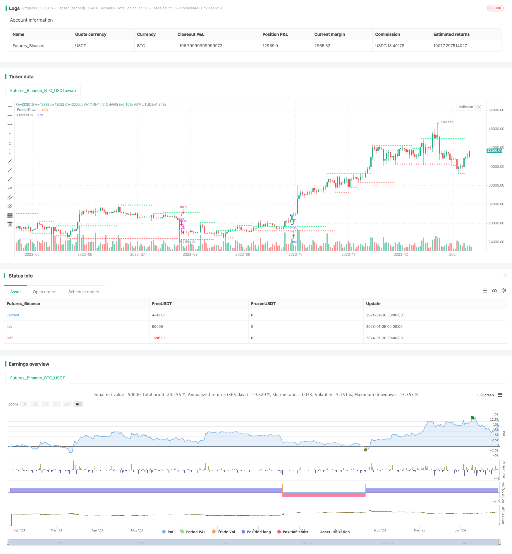
/*backtest
start: 2023-01-25 00:00:00
end: 2024-01-31 00:00:00
period: 1d
basePeriod: 1h
exchanges: [{"eid":"Futures_Binance","currency":"BTC_USDT"}]
*/

//@version=2
strategy("Best Rabbit Strategy", shorttitle="Rabbit God",overlay=true)
Length = input(10, minval=1)
xPrice = close
xvnoise = abs(xPrice - xPrice[1])
Fastend = input(2)
Slowend = input(30)
nfastend = 2/(Fastend + 1)
nslowend = 2/(Slowend + 1)
nsignal = abs(xPrice - xPrice[Length])
nnoise = sum(xvnoise, Length)
nefratio = iff(nnoise != 0, nsignal / nnoise, 0)
nsmooth = pow(nefratio * (nfastend - nslowend) + nslowend, 2)
nAMA = nz(nAMA[1]) + nsmooth * (xPrice - nz(nAMA[1]))

Length2 = input(10, minval=1)
xPrice2 = close
xvnoise2 = abs(xPrice2 - xPrice2[1])
Fastend2 = input(4)
Slowend2 = input(24)
nfastend2 = 2/(Fastend2 + 1)
nslowend2 = 2/(Slowend2 + 1)
nsignal2 = abs(xPrice2 - xPrice2[Length2])
nnoise2 = sum(xvnoise, Length2)
nefratio2 = iff(nnoise2 != 0, nsignal2 / nnoise2, 0)
nsmooth2 = pow(nefratio2 * (nfastend2 - nslowend2) + nslowend2, 2)
nAMA2 = nz(nAMA2[1]) + nsmooth2 * (xPrice2 - nz(nAMA2[1]))

price = input(hl2)
len = input(defval=7,minval=1)
FC = input(defval=4,minval=1)
SC = input(defval=300,minval=1)
len1 = len/2
w = log(2/(SC+1))
H1 = highest(high,len1)
L1 = lowest(low,len1)
N1 = (H1-L1)/len1
H2 = highest(high,len)[len1]
L2 = lowest(low,len)[len1]
N2 = (H2-L2)/len1
H3 = highest(high,len)
L3 = lowest(low,len)
N3 = (H3-L3)/len
dimen1 = (log(N1+N2)-log(N3))/log(2)
dimen = iff(N1>0 and N2>0 and N3>0,dimen1,nz(dimen1[1]))
alpha1 = exp(w*(dimen-1))
oldalpha = alpha1>1?1:(alpha1<0.01?0.01:alpha1)
oldN = (2-oldalpha)/oldalpha
N = (((SC-FC)*(oldN-1))/(SC-1))+FC
alpha_ = 2/(N+1)
alpha = alpha_<2/(SC+1)?2/(SC+1):(alpha_>1?1:alpha_)
out = (1-alpha)*nz(out[1]) + alpha*price

price2 = input(hl2)
len2 = input(defval=31,minval=1)
FC2 = input(defval=40,minval=1)
SC2 = input(defval=300,minval=1)
len12 = len2/2
w2 = log(2/(SC2+1))
H12 = highest(high,len12)
L12 = lowest(low,len12)
N12 = (H1-L1)/len12
H22 = highest(high,len2)[len12]
L22 = lowest(low,len2)[len12]
N22 = (H22-L22)/len12
H32 = highest(high,len2)
L32 = lowest(low,len2)
N32 = (H32-L32)/len2
dimen12 = (log(N12+N22)-log(N32))/log(2)
dimen2 = iff(N12>0 and N22>0 and N32>0,dimen12,nz(dimen12[1]))
alpha12 = exp(w*(dimen2-1))
oldalpha2 = alpha12>1?1:(alpha12<0.01?0.01:alpha12)
oldN2 = (2-oldalpha2)/oldalpha2
N4 = (((SC2-FC2)*(oldN2-1))/(SC2-1))+FC2
alpha_2 = 2/(N4+1)
alpha2 = alpha_2<2/(SC2+1)?2/(SC2+1):(alpha_2>1?1:alpha_2)
out2 = (1-alpha2)*nz(out2[1]) + alpha2*price2

tf = input(title="Resolution",  defval = "current")
vamp = input(title="VolumeMA",  defval=6)
vam = sma(volume, vamp)

up = high[3]>high[4] and high[4]>high[5] and high[2]<high[3] and high[1]<high[2] and volume[3]>vam[3]
down = low[3]<low[4] and low[4]<low[5] and low[2]>low[3] and low[1]>low[2] and volume[3]>vam[3]
fractalup =  up ? high[3] : fractalup[1]
fractaldown = down ? low[3] : fractaldown[1]

fuptf = request.security(syminfo.tickerid,tf == "current" ? timeframe.period : tf, fractalup)
fdowntf = request.security(syminfo.tickerid,tf == "current" ? timeframe.period : tf, fractaldown)

plot(fuptf, "FractalUp", color=lime, linewidth=1, style=cross, transp=0, offset =-3, join=false)
plot(fdowntf, "FractalDown", color=red, linewidth=1, style=cross, transp=0, offset=-3, join=false)

buyEntry= nAMA[0]>nAMA2[0] and out[0]>out2[0]
sellEntry= nAMA[0]<nAMA2[0] and out[0]<out2[0]

if (buyEntry)
    strategy.entry("Buy", strategy.long, comment="Long Position Entry")


if (sellEntry)
    strategy.entry("Sell", strategy.short, comment="Short Position Entry")