概述
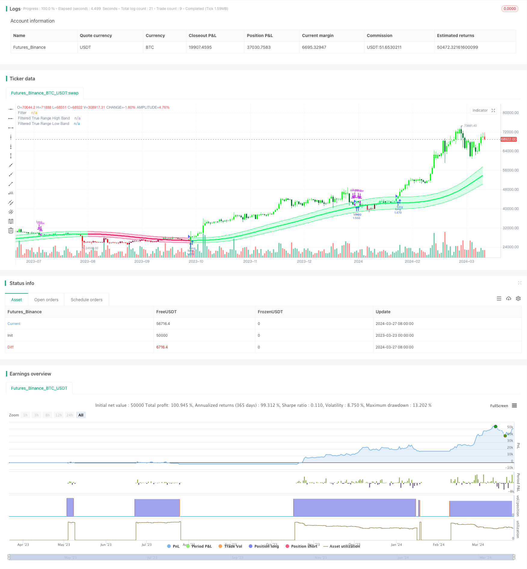
Gaussian Channel趋势追踪策略是一个基于Gaussian Channel指标的趋势跟踪交易策略。该策略旨在捕捉市场的主要趋势,在上升趋势中买入并持有头寸,在下降趋势中平仓观望。策略使用Gaussian Channel指标来识别趋势的方向和强度,通过分析价格与通道上下轨的关系来确定买卖时机。策略的主要目标是在趋势持续期间获得尽可能多的利润,同时尽量避免在震荡市中频繁交易。
策略原理
Gaussian Channel趋势追踪策略的核心是Gaussian Channel指标,该指标由Ehlers提出,是一种利用高斯滤波技术和真实范围(True Range)相结合的趋势分析工具。指标首先根据样本周期和极点数计算β和α值,然后对数据进行滤波处理,得到平滑曲线(中轨)。接着,策略使用平滑后的真实范围乘以一个倍数,得到上下通道。当价格上穿/下穿通道上轨/下轨时,产生买入/卖出信号。此外,策略还提供了降低指标延迟的功能,以及快速反应模式。
策略优势
- 趋势跟踪:该策略善于捕捉市场主要趋势,在趋势方向进行投资,有助于获得长期稳定的收益。
- 减少交易频率:策略只在确认趋势时入场,趋势持续期间保持持仓,从而减少了不必要的交易次数和交易成本。
- 降低延迟:通过降低延迟模式和快速反应模式,策略可以更及时地对市场变化做出反应。
- 参数灵活:用户可以根据自己的需求调整策略参数,如样本周期、极点数、真实范围倍数等,以优化策略表现。
策略风险
- 参数优化风险:不恰当的参数设置可能导致策略表现不佳。建议在不同市场环境下进行参数优化和回测,以找到最佳参数组合。
- 趋势转折风险:当市场趋势发生突然转折时,策略可能会产生较大回撤。可以通过设置止损或引入其他指标来控制风险。
- 震荡市风险:在震荡市场中,策略可能会出现频繁的交易信号,导致收益受损。可以通过优化参数或结合其他技术指标来过滤信号。
策略优化方向
- 引入其他技术指标:结合其他趋势类或震荡类指标,如MACD、RSI等,以提高信号准确性和可靠性。
- 动态参数优化:根据市场状态的变化,动态调整策略参数,以适应不同的市场环境。
- 加入风险控制模块:设置合理的止损和止盈规则,控制单笔交易风险和总体回撤水平。
- 多时间框分析:结合不同时间周期的信号,如日线、4小时线等,以获取更全面的市场信息。
总结
Gaussian Channel趋势追踪策略是一个基于高斯滤波技术的趋势跟踪交易策略,通过捕捉市场主要趋势来获取长期稳定收益。策略使用Gaussian Channel指标来识别趋势方向和强度,同时提供降低延迟和快速反应的功能。策略的优势在于良好的趋势跟踪能力和较低的交易频率,但同时也面临参数优化、趋势转折和震荡市等风险。未来可以通过引入其他技术指标、动态参数优化、加入风险控制模块和多时间框分析等方式对策略进行优化,以进一步提高其稳健性和盈利能力。
策略源码
/*backtest
start: 2023-03-23 00:00:00
end: 2024-03-28 00:00:00
period: 1d
basePeriod: 1h
exchanges: [{"eid":"Futures_Binance","currency":"BTC_USDT"}]
*/

//@version=5
strategy(title="Gaussian Channel Strategy v2.0", overlay=true, calc_on_every_tick=false, initial_capital=1000, default_qty_type=strategy.percent_of_equity, default_qty_value=100, commission_type=strategy.commission.percent, commission_value=0.1, slippage=3)

//-----------------------------------------------------------------------------------------------------------------------------------------------------------------
// Gaussian Channel Indicaor - courtesy of @DonovanWall
//-----------------------------------------------------------------------------------------------------------------------------------------------------------------

// Date condition inputs
startDate = input(timestamp("1 January 2018 00:00 +0000"), "Date Start", group="Main Algo Settings")
endDate = input(timestamp("1 January 2060 00:00 +0000"), "Date Start", group="Main Algo Settings")
timeCondition = true

// This study is an experiment utilizing the Ehlers Gaussian Filter technique combined with lag reduction techniques and true range to analyze trend activity.
// Gaussian filters, as Ehlers explains it, are simply exponential moving averages applied multiple times.
// First, beta and alpha are calculated based on the sampling period and number of poles specified. The maximum number of poles available in this script is 9.
// Next, the data being analyzed is given a truncation option for reduced lag, which can be enabled with "Reduced Lag Mode".
// Then the alpha and source values are used to calculate the filter and filtered true range of the dataset.
// Filtered true range with a specified multiplier is then added to and subtracted from the filter, generating a channel.
// Lastly, a one pole filter with a N pole alpha is averaged with the filter to generate a faster filter, which can be enabled with "Fast Response Mode".

// Custom bar colors are included.

// Note: Both the sampling period and number of poles directly affect how much lag the indicator has, and how smooth the output is.
//      Larger inputs will result in smoother outputs with increased lag, and smaller inputs will have noisier outputs with reduced lag.
//      For the best results, I recommend not setting the sampling period any lower than the number of poles + 1. Going lower truncates the equation.

//-----------------------------------------------------------------------------------------------------------------------------------------------------------------
// Updates:
// Huge shoutout to @e2e4mfck for taking the time to improve the calculation method!
// -> migrated to v4
// -> pi is now calculated using trig identities rather than being explicitly defined.
// -> The filter calculations are now organized into functions rather than being individually defined.
// -> Revamped color scheme.

//-----------------------------------------------------------------------------------------------------------------------------------------------------------------
// Functions - courtesy of @e2e4mfck
//-----------------------------------------------------------------------------------------------------------------------------------------------------------------

// Filter function
f_filt9x (_a, _s, _i) =>
    int _m2 = 0, int _m3 = 0, int _m4 = 0, int _m5 = 0, int _m6 = 0,
    int _m7 = 0, int _m8 = 0, int _m9 = 0, float _f = .0, _x = (1 - _a)
    // Weights.
    // Initial weight _m1 is a pole number and equal to _i
    _m2 := _i == 9 ? 36  : _i == 8 ? 28 : _i == 7 ? 21 : _i == 6 ? 15 : _i == 5 ? 10 : _i == 4 ? 6 : _i == 3 ? 3 : _i == 2 ? 1 : 0
    _m3 := _i == 9 ? 84  : _i == 8 ? 56 : _i == 7 ? 35 : _i == 6 ? 20 : _i == 5 ? 10 : _i == 4 ? 4 : _i == 3 ? 1 : 0
    _m4 := _i == 9 ? 126 : _i == 8 ? 70 : _i == 7 ? 35 : _i == 6 ? 15 : _i == 5 ? 5  : _i == 4 ? 1 : 0
    _m5 := _i == 9 ? 126 : _i == 8 ? 56 : _i == 7 ? 21 : _i == 6 ? 6  : _i == 5 ? 1  : 0
    _m6 := _i == 9 ? 84  : _i == 8 ? 28 : _i == 7 ? 7  : _i == 6 ? 1  : 0
    _m7 := _i == 9 ? 36  : _i == 8 ? 8  : _i == 7 ? 1  : 0
    _m8 := _i == 9 ? 9   : _i == 8 ? 1  : 0
    _m9 := _i == 9 ? 1   : 0
    // filter
    _f :=   math.pow(_a, _i) * nz(_s) +
      _i  *     _x      * nz(_f[1])      - (_i >= 2 ?
      _m2 * math.pow(_x, 2)  * nz(_f[2]) : 0) + (_i >= 3 ?
      _m3 * math.pow(_x, 3)  * nz(_f[3]) : 0) - (_i >= 4 ?
      _m4 * math.pow(_x, 4)  * nz(_f[4]) : 0) + (_i >= 5 ?
      _m5 * math.pow(_x, 5)  * nz(_f[5]) : 0) - (_i >= 6 ?
      _m6 * math.pow(_x, 6)  * nz(_f[6]) : 0) + (_i >= 7 ?
      _m7 * math.pow(_x, 7)  * nz(_f[7]) : 0) - (_i >= 8 ?
      _m8 * math.pow(_x, 8)  * nz(_f[8]) : 0) + (_i == 9 ?
      _m9 * math.pow(_x, 9)  * nz(_f[9]) : 0)

// 9 var declaration fun
f_pole (_a, _s, _i) =>
    _f1 =            f_filt9x(_a, _s, 1),      _f2 = (_i >= 2 ? f_filt9x(_a, _s, 2) : 0), _f3 = (_i >= 3 ? f_filt9x(_a, _s, 3) : 0)
    _f4 = (_i >= 4 ? f_filt9x(_a, _s, 4) : 0), _f5 = (_i >= 5 ? f_filt9x(_a, _s, 5) : 0), _f6 = (_i >= 6 ? f_filt9x(_a, _s, 6) : 0)
    _f7 = (_i >= 2 ? f_filt9x(_a, _s, 7) : 0), _f8 = (_i >= 8 ? f_filt9x(_a, _s, 8) : 0), _f9 = (_i == 9 ? f_filt9x(_a, _s, 9) : 0)
    _fn = _i == 1 ? _f1 : _i == 2 ? _f2 : _i == 3 ? _f3 :
      _i == 4     ? _f4 : _i == 5 ? _f5 : _i == 6 ? _f6 :
      _i == 7     ? _f7 : _i == 8 ? _f8 : _i == 9 ? _f9 : na
    [_fn, _f1]

//-----------------------------------------------------------------------------------------------------------------------------------------------------------------
// Inputs
//-----------------------------------------------------------------------------------------------------------------------------------------------------------------

// Source
src = input(defval=hlc3, title="Source")

// Poles
int N = input.int(defval=4, title="Poles", minval=1, maxval=9)

// Period
int per = input.int(defval=144, title="Sampling Period", minval=2)

// True Range Multiplier
float mult = input.float(defval=1.414, title="Filtered True Range Multiplier", minval=0)

// Lag Reduction
bool modeLag  = input.bool(defval=false, title="Reduced Lag Mode")
bool modeFast = input.bool(defval=false, title="Fast Response Mode")

//-----------------------------------------------------------------------------------------------------------------------------------------------------------------
// Definitions
//-----------------------------------------------------------------------------------------------------------------------------------------------------------------

// Beta and Alpha Components
beta  = (1 - math.cos(4*math.asin(1)/per)) / (math.pow(1.414, 2/N) - 1)
alpha = - beta + math.sqrt(math.pow(beta, 2) + 2*beta)

// Lag
lag = (per - 1)/(2*N)

// Data
srcdata = modeLag ? src + (src - src[lag]) : src
trdata  = modeLag ? ta.tr(true) + (ta.tr(true) - ta.tr(true)[lag]) : ta.tr(true)

// Filtered Values
[filtn, filt1]     = f_pole(alpha, srcdata, N)
[filtntr, filt1tr] = f_pole(alpha, trdata,  N)

// Lag Reduction
filt   = modeFast ? (filtn + filt1)/2 : filtn
filttr = modeFast ? (filtntr + filt1tr)/2 : filtntr

// Bands
hband = filt + filttr*mult
lband = filt - filttr*mult

// Colors
color1   = #0aff68
color2   = #00752d
color3   = #ff0a5a
color4   = #990032
fcolor   = filt > filt[1] ? #0aff68 : filt < filt[1] ? #ff0a5a : #cccccc
barcolor = (src > src[1]) and (src > filt) and (src < hband) ? #0aff68 : (src > src[1]) and (src >= hband) ? #0aff1b : (src <= src[1]) and (src > filt) ? #00752d :
           (src < src[1]) and (src < filt) and (src > lband) ? #ff0a5a : (src < src[1]) and (src <= lband) ? #ff0a11 : (src >= src[1]) and (src < filt) ? #990032 : #cccccc

//-----------------------------------------------------------------------------------------------------------------------------------------------------------------
// Outputs
//-----------------------------------------------------------------------------------------------------------------------------------------------------------------

// Filter Plot
filtplot = plot(filt, title="Filter", color=fcolor, linewidth=3)

// Band Plots
hbandplot = plot(hband, title="Filtered True Range High Band", color=fcolor)
lbandplot = plot(lband, title="Filtered True Range Low Band", color=fcolor)

// Channel Fill
fill(hbandplot, lbandplot, title="Channel Fill", color=color.new(fcolor, 80))

// Bar Color
barcolor(barcolor)

longCondition = ta.crossover(close, hband) and timeCondition
closeAllCondition = ta.crossunder(close, hband) and timeCondition

if longCondition
    strategy.entry("long", strategy.long)

if closeAllCondition
    strategy.close("long")