Momentum Adaptive Gaussian Channel Multi-Period Strategy

Overview
This strategy is a momentum trading system based on Gaussian channels and stochastic RSI indicators, combined with seasonal filtering and volatility management. It identifies market trends through adaptive Gaussian channels, confirms momentum using stochastic RSI, and executes trades within specific seasonal windows. The system also incorporates ATR-based position management to control risk exposure per trade.
Strategy Principles
The core of the strategy is a price channel built on multi-pole Gaussian filters. The channel is constructed by calculating Gaussian filtered values of HLC3 prices and combining them with filtered true range (TR) results to form dynamic upper and lower bands. Trade signals are generated when the following conditions are met:
- Price breaks above the upper band and the main filter trend is up
- Stochastic RSI indicates overbought conditions
- Current time is within the preset seasonal window
- Position size is dynamically calculated based on ATR
Exit signals are triggered when price falls below the lower band. The entire system enhances trading stability through multiple filtering mechanisms.
Strategy Advantages
- Gaussian filters provide excellent noise reduction capability, effectively capturing genuine market trends
- Multi-pole design offers more precise price channel boundaries
- Integration of momentum and trend indicators improves signal reliability
- Seasonal filtering helps avoid unfavorable market conditions
- Dynamic position management ensures consistency in risk exposure
- System parameters can be optimized for different market conditions
Strategy Risks
- Complex Gaussian filter calculations may lead to execution delays
- Multiple filtering conditions might miss important trading opportunities
- System is sensitive to parameter settings, requiring careful optimization
- Fixed seasonal windows may not adapt to changing market environments
- ATR-based position control might be too conservative during high volatility periods
Optimization Directions
- Introduce adaptive seasonal windows that dynamically adjust trading times based on market conditions
- Optimize Gaussian filter calculations to reduce execution delays
- Add market volatility adjustment mechanisms to modify filtering conditions in different market environments
- Develop more flexible position management systems to balance risk and reward
- Incorporate multi-timeframe analysis to improve signal reliability
Summary
This is a well-constructed trend following system that enhances trading stability through multiple layers of filtering and risk management mechanisms. While there is room for optimization, the overall design philosophy aligns with modern quantitative trading requirements. The key to strategy success lies in precise parameter adjustment and adaptability to market conditions.
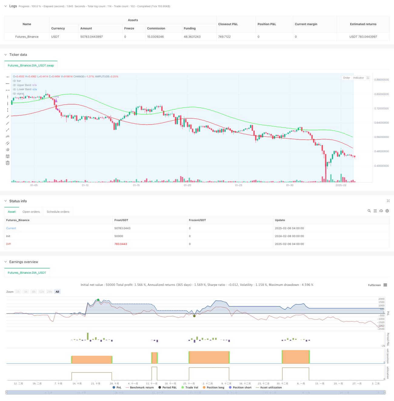
/*backtest
start: 2024-02-08 00:00:00
end: 2025-02-06 08:00:00
period: 4h
basePeriod: 4h
exchanges: [{"eid":"Futures_Binance","currency":"DIA_USDT"}]
*/

//@version=6
strategy("Demo GPT - Gold Gaussian Strategy", overlay=true, commission_type=strategy.commission.percent, commission_value=0.1)

// ====== INPUTS ======- 1