
Overview
This strategy is a trend following trading system based on Gaussian filtering and StochRSI indicator. It uses Gaussian channels to identify market trends and combines StochRSI indicator's overbought/oversold zones to optimize entry timing. The system employs polynomial fitting to construct Gaussian channels, tracking price trends through dynamic adjustment of upper and lower bands.
Strategy Principle
The core of the strategy is the price channel built on Gaussian filtering algorithm. Key implementation steps include:
- Implementing 9th-order Gaussian filtering using polynomial function f_filt9x with pole optimization
- Calculating main filter line and volatility channel based on HLC3 price
- Introducing reducedLag mode to decrease filtering delay and fastResponse mode to improve response speed
- Utilizing StochRSI indicator's overbought/oversold zones (80/20) for trade signals
- Generating long signals when Gaussian channel trends upward and price breaks above upper band, combined with StochRSI conditions
- Closing positions when price falls below upper band
Strategy Advantages
- Excellent noise reduction capability through Gaussian filtering
- Smooth trend tracking via polynomial fitting, reducing false signals
- Supports delay optimization and fast response modes for flexible market adaptation
- Improved entry timing through StochRSI indicator integration
- Dynamic channel width adapting to market volatility changes
Strategy Risks
- Inherent lag in Gaussian filtering may lead to delayed entries or exits
- May generate frequent trading signals in ranging markets, increasing transaction costs
- StochRSI indicator might produce lagging signals under certain market conditions
- Complex parameter optimization process requiring readjustment for different markets
- High computational resource requirements leading to potential real-time calculation delays
Optimization Directions
- Introduce adaptive parameter optimization based on market conditions
- Add market environment recognition for different parameter combinations
- Optimize Gaussian filtering algorithm to further reduce calculation delay
- Incorporate additional technical indicators for cross-validation
- Develop intelligent stop-loss mechanisms for improved risk control
Summary
The strategy achieves effective market trend tracking through the combination of Gaussian filtering and StochRSI indicator. While the system demonstrates strong noise reduction and trend identification capabilities, it faces challenges with latency and parameter optimization. Through continuous improvement and refinement, the strategy shows potential for generating stable returns in actual trading.
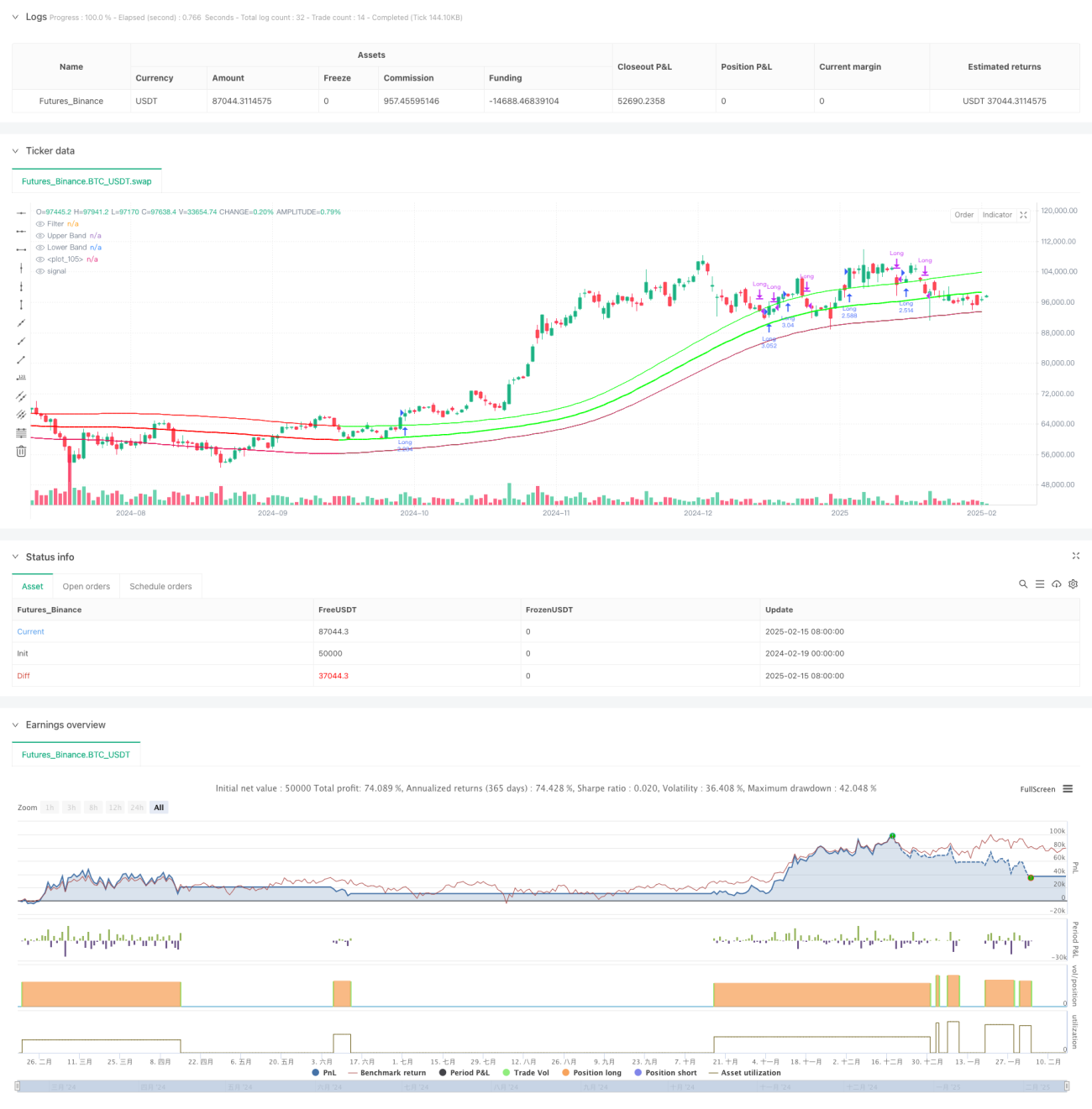
/*backtest
start: 2024-02-19 00:00:00
end: 2025-02-16 08:00:00
period: 1d
basePeriod: 1d
exchanges: [{"eid":"Futures_Binance","currency":"BTC_USDT"}]
*/

//@version=5
strategy(title="Demo GPT - Gaussian Channel Strategy v3.0", overlay=true, commission_type=strategy.commission.percent, commission_value=0.1, slippage=0, default_qty_type=strategy.percent_of_equity, default_qty_value=250)

// ============================================- 1