Overview

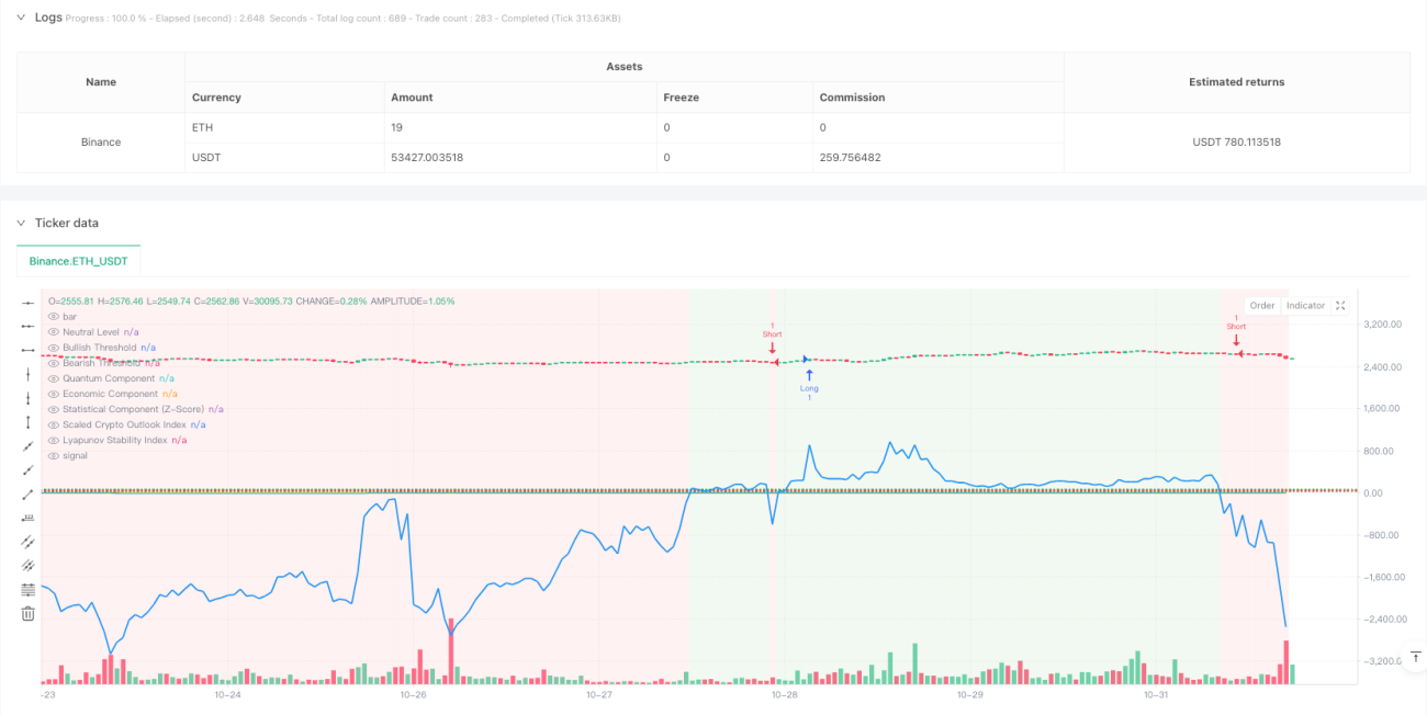
This strategy is an innovative quantitative trading system that integrates principles from quantum mechanics, statistics, and economics. It constructs a comprehensive market analysis framework by combining Simple Moving Average (SMA), Z-Score statistical analysis, quantum oscillation component, economic momentum indicators, and the Lyapunov stability index. The strategy's core generates a Composite Outlook Index (COI) through weighted combinations of these multi-dimensional indicators to guide trading decisions.

Strategy Principles

The strategy is built on five main technical pillars:

1. Statistical analysis module uses SMA and standard deviation to calculate Z-Score, evaluating relative price positions.
2. Quantum component transforms Z-Score into an oscillator, simulating quantum state fluctuations through exponential and sine functions.
3. Economic component measures market momentum using the logarithmic ratio of fast and slow EMAs.
4. Lyapunov index assesses market stability by analyzing the combined stability of quantum and economic components.
5. Composite Outlook Index (COI) integrates all components with different weights to form final trading signals.

Strategy Advantages

1. Multi-dimensional analysis provides more comprehensive market insights, reducing bias from single indicators.
2. Introduction of quantum component brings unique market oscillation perspective, helping capture short-term opportunities.
3. Application of Lyapunov index effectively evaluates market stability, enhancing risk management capabilities.
4. Adjustable weights design allows strategy adaptation to different market environments.
5. Neutral line design in composite index provides clear trading signal boundaries.

Strategy Risks

1. Multiple indicators may lead to signal lag, affecting entry timing.
2. Parameter optimization may result in overfitting risk.
3. Quantum component may generate too frequent signals in high volatility markets.
4. Economic component may produce misleading signals in ranging markets.
5. Proper stop-loss settings are necessary for risk control.

Strategy Optimization Directions

1. Introduce adaptive weight system to dynamically adjust component weights based on market conditions.
2. Add volatility filters to adjust signal sensitivity during high volatility periods.
3. Integrate market sentiment indicators to provide additional confirmation signals.
4. Develop dynamic stop-loss mechanisms to adjust stop-loss levels based on market conditions.
5. Add time filters to avoid opening positions during unfavorable trading periods.

Summary

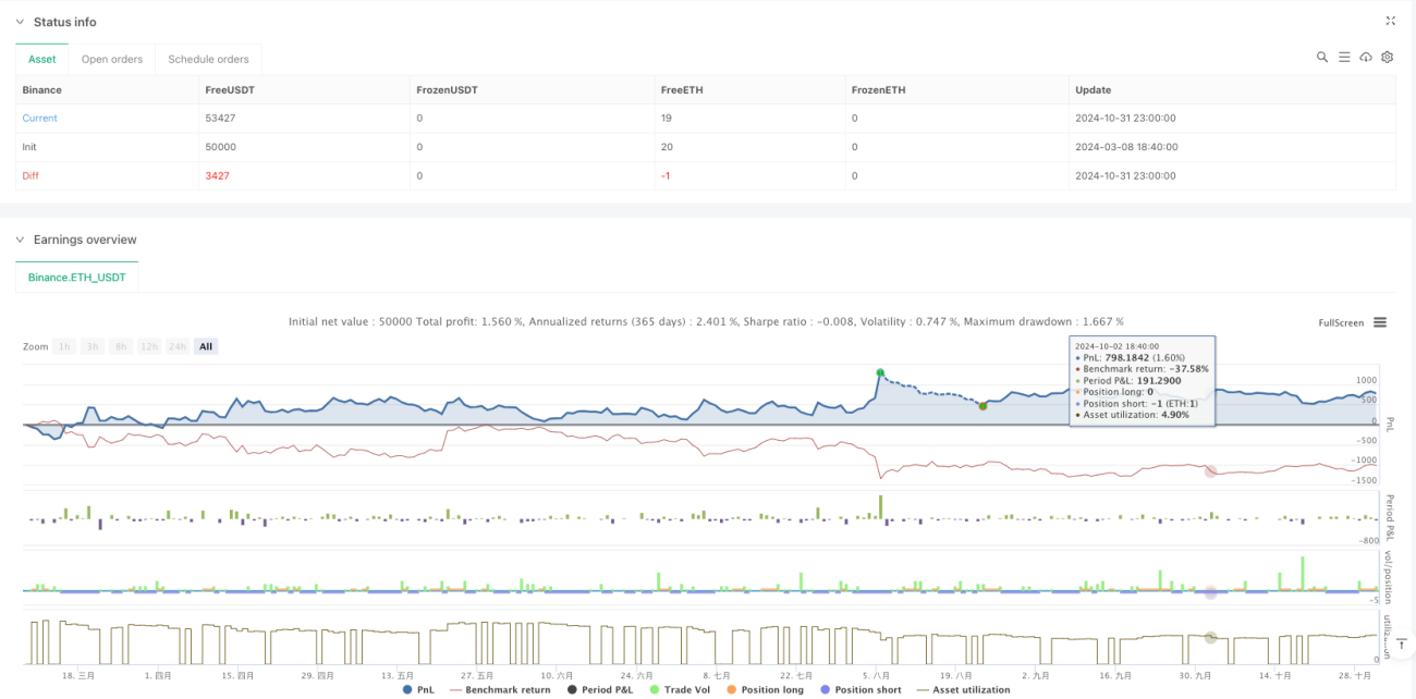
This is an innovative quantitative trading strategy that builds a comprehensive market analysis framework by integrating multi-disciplinary theories. While there are areas for optimization, its multi-dimensional analysis approach provides unique perspectives for trading decisions. Through continuous optimization and risk management improvements, the strategy shows promise for maintaining stable performance across different market environments.