

A Comparative Online Learning Experiment Based on FMZ Rust
Online learning is easily presented as a natural advantage in quantitative research: markets are non-stationary, so models should continuously absorb new data.
That line of reasoning is only half complete.
Faster model updates may indeed help a model move away from historical relationships that have already broken down. But the same update mechanism can also write short-term random fluctuations into the parameters more quickly. For a trading strategy, the latter does not merely appear as unstable predictions. It also turns into higher turnover, greater sensitivity to costs, and stronger path dependence.
This article therefore does not attempt to prove that “online models are better than fixed models.” The experiment asks a more specific question:
When the model structure, features, trading rules, and cost assumptions are held completely constant, how does changing the speed at which the model absorbs new samples affect out-of-sample loss, parameter stability, turnover, and simulated equity?
To avoid mixing model differences with differences in the backtesting environment, four models run in parallel inside the same Rust strategy process. They read the same bars and use the same features and simulated execution rules. The strategy does not send orders to an exchange; it maintains four shadow accounts only.
This article includes one actual backtest to verify whether the time alignment, label distribution, predictive loss, turnover, and trading costs behave as expected. However, a single backtest is not treated as a general conclusion. The main value of the strategy is still to establish a reproducible comparison framework.
1. Research Question: Update Speed Is Itself a Source of Model Risk
Online learning usually follows the sequence “predict first, observe the label, then update.” When sample \(t\) arrives, the model first makes a prediction using its current parameters. After the true outcome becomes available, the loss is calculated and the parameters are updated.
The advantage of this approach is that new information can be absorbed incrementally without repeatedly saving and retraining on the entire history. The problem is that every new sample immediately affects the parameters.
The update mechanism can be understood as a continuous speed axis:
text
Never update
── Periodic rolling retraining
── Update after loss deterioration
── Update after every bar
── Update after every tick
The farther left a model sits, the more stable its parameters are, but the slower it responds to structural change. The farther right it sits, the more flexible it becomes—and the more easily it can be pushed around by short-term noise.
The experiment therefore proposes three hypotheses to test in advance, rather than assuming an answer:
- Per-bar online updates may shorten the model’s recovery time after a regime change.
- The same mechanism may also amplify parameter fluctuations, signal reversals, and trading costs.
- Model performance may not improve monotonically with update frequency; an intermediate speed may be more stable.
2. Experimental Design: Change Only How the Model Absorbs New Samples
All four models share the same initialized parameters.
| Model | Update Method | Research Interpretation |
|---|---|---|
| Fixed model | No further updates after initialization | Observe how quickly the historical relationship naturally decays |
| Per-bar online | Perform one gradient update whenever a new label becomes available | Fastest sample absorption |
| Rolling retraining | Retrain from scratch on the most recent window after a fixed number of bars | Reduce the immediate influence of a single sample |
| Error-gated | When recent Log Loss deteriorates materially, update slowly on a small batch of recent samples | Add a threshold between stability and adaptation |
The fourth group can only be called an error-gated update mechanism. It cannot be described as a strict concept-drift detector.
An increase in predictive loss may result from a change in the conditional distribution, but it may also come from higher volatility, outliers, label randomness, or poor model calibration. This article uses loss deterioration only as an engineering trigger. It does not infer from that trigger alone that concept drift has occurred in the market.
To keep the comparison as clean as possible, all four models use exactly the same:
- initial training samples;
- features and standardization parameters;
- logistic-regression structure;
- long and short probability thresholds;
- return calculation method;
- one-way turnover-cost assumption.
The four simulated accounts are also settled synchronously on the same bar. As a result, differences in the outcomes mainly come from the update mechanism rather than from data segmentation, API timing, or backtest-matching differences.
3. Time Alignment: Resolve Look-Ahead Bias and Execution Assumptions First
The easiest place to make a mistake in an online model is not the gradient formula, but sample timing.
After bar \(t\) closes, this experiment calculates features \(x_t\) and predicts the open-to-close direction of bar \(t+1\):

Strictly speaking, class 0 means non-up, because a bar with an opening price equal to its closing price is also encoded as 0.
The label function is:
rust
fn make_label(
bars: &[Bar],
feature_index: usize,
) -> f64 {
let next_bar =
bars[feature_index + 1];
if next_bar.close > next_bar.open {
1.0
} else {
0.0
}
}
The process is:
            text

            Bar t closes
        ↓
Calculate x_t and predict the direction of bar t+1
        ↓
Assume a position is established near the open of bar t+1
        ↓
Bar t+1 closes, producing the label and open-to-close return
        ↓
Evaluate the original prediction first, then allow the model to update
This definition does not assume that the strategy can wait until a closing price is known and still trade at the closing price of bar \(t\).
The simulated account uses the open-to-close return of bar \(t+1\):
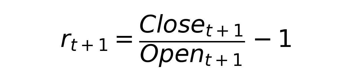
This is still a simplified model. A real order may not fill at the opening price of the next bar, and order-book impact, latency, and slippage will not remain fixed. The cost in the code is only a standardized stress-test assumption and does not represent the actual fee schedule of any exchange.
3.1 Identifying Completed Bars Separately in Backtesting and Live Trading
The first version of the strategy used the current time in every environment to determine whether a bar had finished. In the actual backtest, this caused a still-forming bar to be treated prematurely as a completed sample. A large number of bars therefore appeared with Open == Close, and model accuracy became abnormally close to 100%.
The corrected version uses IsVirtual() to distinguish between runtime environments:
- In backtesting, it conservatively uses the second-to-last bar in the market-data array.
- In live trading, it checks whether the start time of the last bar plus the bar duration is no later than the current time.
- If the final bar returned by the live API has not finished, the function falls back to the second-to-last bar.
            rust

            fn latest_closed_index(
    bars: &[Bar],
    is_backtest: bool,
    bar_seconds: i64,
) -> Option<usize> {
    if bars.len() < 2 {
        return None;
    }

    if is_backtest {
        return Some(bars.len() - 2);
    }

    let last_index = bars.len() - 1;
    let period_ms = bar_seconds * 1000;
    let current_time_ms =
        (UnixNano() / 1_000_000) as i64;

    if bars[last_index].time + period_ms
        <= current_time_ms
    {
        Some(last_index)
    } else {
        Some(last_index - 1)
    }
}
The cost of processing one fewer bar is far smaller than the cost of mistakenly treating incomplete data as a label.
3.2 Test-Then-Train
Whenever a new label appears, the processing order is strictly maintained as follows:
- Use the previously stored prediction to calculate accuracy and Log Loss.
- Use the previously determined position to calculate the return on the current bar.
- Add the current sample to the training data.
- Update each model according to its own rule.
- Use the current completed bar to generate the prediction for the next bar.
In other words, test first and train afterward. The current sample is not fed into the model before the same sample is used to evaluate it.
4. Model: Simple Logistic Regression Is Enough for This Experiment
This article does not use a neural network or a tree model. It uses logistic regression with L2 regularization:
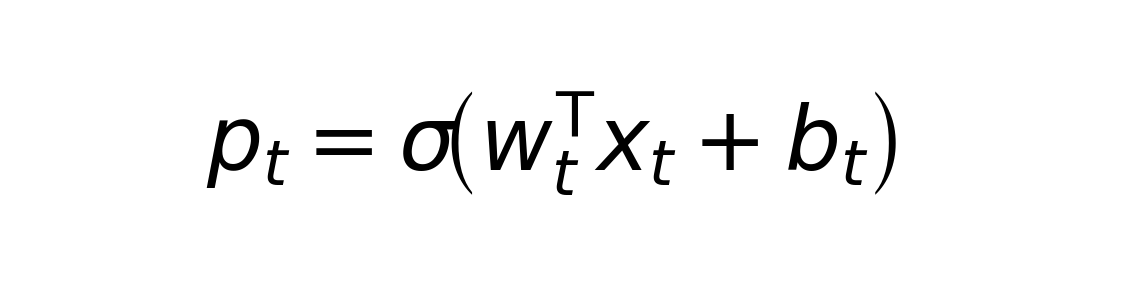
Here, \(p_t\) is the estimated probability that the next bar will rise.
The per-bar update uses the stochastic gradient corresponding to binary cross-entropy:

The equation above shows only the weight terms. The bias \(b\) is also updated in the code, but no L2 regularization is applied to it.
            rust

            fn predict(
    &self,
    features: &[f64; N_FEATURES],
) -> f64 {
    let mut linear_value = self.bias;

    for j in 0..N_FEATURES {
        linear_value +=
            self.weights[j] * features[j];
    }

    Self::sigmoid(linear_value)
}

fn update(
    &mut self,
    features: &[f64; N_FEATURES],
    label: f64,
    learning_rate_scale: f64,
) {
    let probability = self.predict(features);
    let error = probability - label;
    let step =
        self.learning_rate
            * learning_rate_scale;

    for j in 0..N_FEATURES {
        let gradient = clip(
            error * features[j]
                + self.l2_penalty
                    * self.weights[j],
            -5.0,
            5.0,
        );
        self.weights[j] -= step * gradient;
    }

    self.bias -=
        step * clip(error, -1.0, 1.0);

    self.updates += 1;
}
Choosing a simple model does not imply that logistic regression is sufficient to describe the market. The purpose is to reduce confounding factors in the experiment.
If the network structure, training epochs, number of features, and update frequency are all changed at the same time, it becomes difficult to determine where the difference in returns comes from. Parameter changes in a linear model can be measured directly, making it easier to observe whether “model adaptation” is accompanied by excessive weight drift.
The code also clips individual gradients and standardized features. The purpose is not to improve returns, but to prevent an extreme bar from pushing the parameters too far in a single update.
5. Features: Retain Only Basic Price-Structure and Volume Information
The model uses eight features:
- one-bar log return;
- log return of the candle body;
- log range between the high and low;
- relative upper-wick length;
- relative lower-wick length;
- log change in volume;
- three-bar momentum;
- realized volatility of returns over the most recent five bars.
No derived indicators such as RSI, MACD, or moving-average crossovers are included, and the model does not use dozens of lagged terms.
The main part of the feature calculation is shown below:
            rust

            fn raw_features(
    bars: &[Bar],
    index: usize,
) -> [f64; N_FEATURES] {
    let current = bars[index];
    let previous = bars[index - 1];
    let epsilon = 1e-12;

    let log_return_1 =
        (current.close.max(epsilon)
            / previous.close.max(epsilon))
            .ln();

    let candle_body =
        (current.close.max(epsilon)
            / current.open.max(epsilon))
            .ln();

    let range =
        (current.high.max(epsilon)
            / current.low.max(epsilon))
            .ln();

    let upper_wick =
        (current.high
            - current.open.max(current.close))
            .max(0.0)
            / current.open.max(epsilon);

    let lower_wick =
        (current.open.min(current.close)
            - current.low)
            .max(0.0)
            / current.open.max(epsilon);

    let volume_change =
        ((current.volume + epsilon)
            / (previous.volume + epsilon))
            .ln();

    let momentum_3 =
        (current.close.max(epsilon)
            / bars[index - 3]
                .close
                .max(epsilon))
            .ln();

    // Realized volatility of returns over the most recent five bars
    // The full implementation continues the calculation over the same window.

    [
        log_return_1,
        candle_body,
        range,
        upper_wick,
        lower_wick,
        volume_change,
        momentum_3,
        realized_volatility,
    ]
}
The initial samples are divided chronologically into the first 80% and the final 20%. The standardizer fits its means and standard deviations using only the first 80% of the features and then remains fixed. All four models always use the same standardizer.
The standardizer is deliberately not updated online. Otherwise, the per-bar model would receive not only parameter updates but also an additional layer of feature-distribution adaptation, and the comparison would no longer isolate a single variable.
A fixed standardizer helps keep the four models comparable, but it may also produce scale mismatch when the feature distribution changes over a long period. Therefore, the results of this experiment contain the combined effects of model-relationship failure and fixed-standardization scale mismatch. The two effects are not separately identified.
6. Initialization: All Four Models Must Start from the Same Line
By default, the code prepares 320 initial supervised samples.
Initialization is performed in two stages:
- Run six epochs of batch training on the first 80% of samples.
- Process the final 20% one by one using “predict—record loss—update.”
The average pre-update Log Loss produced by the second stage is used as the reference loss for the error-gated model. Only after this segment has been processed is the resulting model used as the shared initial parameter state for all four models.
            rust

            fn fit_initial_model(
    samples: &[Sample],
    split_index: usize,
    config: &Config,
) -> (LogisticModel, f64) {
    let mut model =
        train_model(
            &samples[..split_index],
            config.initial_epochs,
            config,
        );

    let mut loss_sum = 0.0;
    let mut count = 0usize;

    for sample in &samples[split_index..] {
        let probability =
            model.predict(&sample.x);

        loss_sum +=
            log_loss(
                probability,
                sample.y,
            );

        count += 1;

        model.update(
            &sample.x,
            sample.y,
            1.0,
        );
    }

    let baseline_loss =
        if count == 0 {
            0.69314718056
        } else {
            loss_sum / count as f64
        };

    (model, baseline_loss)
}
This treatment resolves two problems.
First, the reference loss is not an in-sample retrospective loss calculated on data the model has already trained on. It is a pre-update loss obtained in chronological order.
Second, all four models begin from the same parameter state, which has already absorbed all initialization samples. This prevents a situation in which the fixed and online models use different initial training data while later differences are still attributed to the update method.
7. Four Update Mechanisms
7.1 Fixed Model
The fixed model no longer modifies its weights after initialization.
It provides the benchmark. If subsequent performance continues to deteriorate, the relationship learned during initialization cannot be stably extrapolated. If the fixed model is instead the most stable, the additional updates have not provided enough incremental information.
It is important to note that a fixed model only means its weights and bias are no longer updated. It does not mean the predicted probability or position remains unchanged. Input features change on every bar, so fixed parameters can still generate frequent turnover.
7.2 Per-Bar Online Model
One gradient update is performed after each label becomes available:
            rust

            online_model.update(
    &previous_features,
    label,
    1.0,
);
This model reacts fastest to a new environment, but it is also the most likely to interpret a short run of accidental samples as a structural change.
The learning rate is the most important risk parameter for this model. The larger the learning rate, the stronger the influence of a new sample on the parameters. This article uses the interface default of 0.02 and performs no in-sample optimization.
7.3 Rolling-Retraining Model
Under the default settings, the rolling model stores the most recent 240 samples. After every 32 new samples, its parameters are reset and the model is retrained from scratch on the samples in the window.
            rust

            if processed_bars
    % config.retrain_every
    == 0
{
    periodic_model =
        retrain_from_window(
            &rolling_samples,
            &config,
        );

    periodic_retrains += 1;
}
This method has two characteristics:
- Old samples are explicitly removed from the training set.
- A single new sample does not immediately change the model. Instead, it takes effect together with a batch of recent samples at the next retraining point.
Its adaptation is delayed, but parameter changes are usually not driven entirely by the final observation in the same way as per-bar updates. Both the rolling window and retraining interval can be adjusted in the strategy interface.
7.4 Error-Gated Model
The gated model maintains an exponential moving average of its own predictive Log Loss:

Only when recent loss exceeds the initialization reference loss by a specified proportion, and the model is not in a cooldown period, does it update at a low learning rate using a small batch of the most recent samples.
            rust

            let current_gated_loss =
    log_loss(
        gated_old_probability,
        label,
    );

gated_loss_ema =
    (1.0 - config.loss_ema_alpha)
        * gated_loss_ema
        + config.loss_ema_alpha
            * current_gated_loss;

let gate_threshold =
    baseline_loss
        * config.gate_loss_multiplier;

if gate_cooldown_left == 0
    && gated_loss_ema > gate_threshold
{
    let batch_start =
        rolling_samples
            .len()
            .saturating_sub(
                config.gate_batch
            );

    for (sample_index, sample)
        in rolling_samples
            .iter()
            .enumerate()
    {
        if sample_index >= batch_start {
            gated_model.update(
                &sample.x,
                sample.y,
                config.gated_lr_scale,
            );
        }
    }

    gate_events += 1;
    gate_cooldown_left =
        config.gate_cooldown;
}
The interface defaults are:
- Loss threshold: 1.10 times the reference loss.
- Update batch: the most recent 32 samples.
- Learning-rate scale: 0.25 times the base learning rate.
- Post-update cooldown: 32 bars.
These values are only unoptimized experimental defaults. Their purpose is to define a repeatable gating rule, not to represent statistically optimal thresholds.
8. Trading Mapping and Costs
Model probabilities are mapped into three positions:
            rust

            fn position_from_probability(
    probability: f64,
    config: &Config,
) -> i32 {
    if probability >= config.long_threshold {
        1
    } else if probability
        <= config.short_threshold
    {
        -1
    } else {
        0
    }
}
The default rule is:
            text

            p >= 0.55: long
p <= 0.45: short
otherwise: flat
The neutral range from 0.45 to 0.55 is intended to reduce the conversion of small probability fluctuations around 0.5 directly into trades.
The position-change amount is defined as:

Therefore:
- flat to long has turnover of 1;
- long to flat has turnover of 1;
- a direct flip from long to short has turnover of 2.
The cost is configured as an interface parameter rather than a hard-coded constant:
            rust

            let cost_bps = float_parameter(
    "CostBps",
    CostBps,
    0.0,
    100.0,
    true,
)?;

cost_per_turnover:
    cost_bps / 10_000.0,
CostBps defaults to 5, meaning that 5 basis points are deducted for each unit of one-way turnover. This is an experimental parameter that can be adjusted in the strategy interface. It does not represent the actual fee rate of any specific exchange.
9. Evaluation Metrics: Do Not Look Only at Accuracy
All four models record the following metrics:
| Metric | Purpose |
|---|---|
| Average Log Loss | Whether probability forecasts become more reliable, rather than merely getting the direction right by chance |
| Directional Accuracy | Basic classification performance at a 0.5 threshold |
| Simulated Net Return | Whether predictions translate into returns under the same trading rules |
| Maximum Drawdown | Whether the update mechanism increases equity-path risk |
| Position Rate | Whether a model appears stable only because it trades less |
| Cumulative Turnover | Sensitivity to trading costs |
| Number of Position Changes | Whether the signal frequently changes its mind |
| Direct Long-Short Flips | Whether the model swings sharply between the two directions |
| Parameter Displacement | Distance between the current parameters and the shared initial model |
Parameter displacement is defined as the Euclidean distance of the differences in the weights and bias. Because the features use the same fixed standardizer, the four models can be compared on a relative basis.
A large parameter displacement is not an error by itself. If the market structure truly changes, the model needs to move. The combination that should raise concern is:
            text

            Parameter displacement rises rapidly
+ Turnover increases materially
+ Log Loss does not improve
+ Net equity after costs deteriorates
This looks more like the model is chasing recent samples than acquiring stable adaptive ability.
10. One Actual Backtest Under the Default Parameters
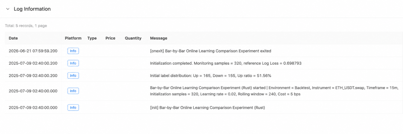
After correcting the completed-bar logic, a baseline backtest was run under the following conditions:
            text

            Instrument: ETH_USDT.swap
Timeframe: 15 minutes
Backtest period: 2025-07-09 to 2026-06-21
Initialization samples: 320
Out-of-sample bars: 33333
Base learning rate: 0.02
Rolling window: 240
One-way turnover cost: 5 bps
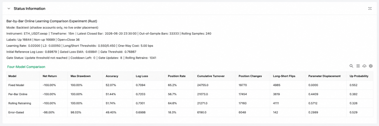
In the out-of-sample statistics, there were 16,644 up labels and 16,689 non-up labels. Among them, 36 bars had identical opening and closing prices. The status panel currently displays the latter category as “down,” but the actual code definition is Close <= Open; the remainder of this article therefore uses the term non-up.
| Model | Accuracy | Log Loss | Position Rate | Cumulative Turnover | Long-Short Flips | Parameter Displacement | Net Return |
|---|---|---|---|---|---|---|---|
| Fixed model | 52.07% | 0.7094 | 65.2% | 24755 | 4985 | 0.0000 | -100.00% |
| Per-bar online | 51.44% | 0.7203 | 56.7% | 21073 | 3619 | 0.4409 | -100.00% |
| Rolling retraining | 51.74% | 0.7301 | 64.6% | 21271 | 4111 | 0.5712 | -100.00% |
| Error-gated | 49.40% | 0.6986 | 18.3% | 6190 | 142 | 0.2989 | -98.00% |
10.1 The Time-Alignment Problem Has Been Corrected
The up and non-up labels are nearly balanced, and model accuracy has returned to 49%–52%. The initialization reference Log Loss is 0.6988. The earlier accuracy close to 100% did indeed come from processing incomplete bars prematurely, not from the model suddenly acquiring extremely strong predictive ability.
10.2 More Frequent Updates Did Not Improve Out-of-Sample Probability Forecasts
For a naive probability model that always outputs 0.5, the Log Loss on every sample is approximately 0.6931.
In this backtest, the average Log Loss of all four models was above that benchmark. The error-gated model was closest to 0.6931, but it still cannot be said that the model had acquired effective predictive ability.
Both per-bar online updating and rolling retraining produced clear parameter displacement, but their Log Loss rose to 0.7203 and 0.7301 respectively, both worse than the fixed model. At least for the current instrument, timeframe, features, and default parameters, more frequent model updates did not improve out-of-sample probability forecasts.
10.3 The Gating Mechanism Reduced Noise Reactions but Did Not Create a Trading Edge
The error-gated model triggered only eight updates. Its cumulative turnover fell to 6,190, and it recorded only 142 direct long-short flips, both markedly lower than the other three models.
This shows that the gating mechanism at least achieved its engineering objective: reducing the frequency with which the model changed its mind because of short-term errors.
However, its post-cost equity still fell by approximately 98%. The correct conclusion is not that “error gating has already become effective,” but rather:
Controlled updating is more stable than unconditional updating, but stability itself has not yet translated into a trading edge.
The final status display of “update threshold not reached” only means that the loss EMA was below the threshold at the end of the backtest. It does not contradict the fact that eight updates were triggered earlier in the historical path.
10.4 A Fixed Model Can Still Generate Frequent Turnover Without Updating Its Parameters
The fixed model’s parameter displacement is 0, yet its cumulative turnover is the highest of all four models.
There is no contradiction. A fixed model only means that the weights and bias no longer change. The input features \(x_t\) are still different on every bar. Fixed parameters combined with changing inputs can still produce changing probabilities and positions.
10.5 Once Equity Approaches Zero, Return Metrics Become Saturated
All four models suffered severe losses under a 5 bps one-way cost. The primary problem was not a single large loss, but the accumulation of substantial turnover across more than 30,000 bars.
Once equity approaches zero, net return and maximum drawdown both approach their limiting values, making it difficult to continue distinguishing the models economically.
A later version should at least add:
- gross return before costs;
- cumulative costs;
- net log return;
- turnover per 1,000 bars;
- multiple cost scenarios at 0, 2, 5, and 10 bps.
These results cannot prove that online learning is ineffective in other markets. They only show that, under the conditions of this experiment, updating the model more frequently did not demonstrate stronger market adaptation. Controlled updating reduced reactions to noise, but the added stability did not translate into a trading edge.
11. Complete Rust Implementation
The complete strategy only reads bars and maintains four models and four simulated accounts in memory. It contains no real order-placement logic.
Strategy Code: Online Bar-by-Bar Learning Comparison Experiment (Rust)
12. How to Tell Whether a Model Is Adapting or Chasing Noise
The online model having the highest equity in a single backtest does not directly prove that online updating is effective. More informative evidence comes from the relationship between metrics and from whether the conclusion can be repeated across different periods.
Case 1: Log Loss Improves Without a Material Increase in Turnover
If the per-bar model reduces Log Loss relatively quickly after a regime change, while parameter displacement stabilizes and cumulative turnover remains close to that of the fixed model, this is stronger evidence of adaptation.
The important point is not that “the parameters moved,” but that predictive quality improved persistently after they moved.
Case 2: Accuracy Improves, but Log Loss and Equity Deteriorate
Accuracy only considers whether the predicted probability crosses 0.5. It does not account for how confident the model is.
A model may increase a probability from 0.51 to 0.90 while remaining directionally correct. But once the prediction is wrong, Log Loss deteriorates significantly. In trading, this kind of overconfidence is also more likely to push a signal across the long and short thresholds.
Therefore, it is not contradictory for the online model to have slightly higher accuracy while showing worse Log Loss, drawdown, and post-cost returns.
Case 3: An Advantage Exists at Zero Cost but Disappears After Costs Are Added
This usually means that online updating generated more marginal signals, but the edge per trade was not large enough to cover trading frictions.
The model may indeed have captured a small amount of short-term predictability, but that predictability did not reach tradable strength. An improvement in gross return cannot be equated with an effective strategy.
Case 4: Rolling Retraining or Gated Updating Is More Stable
If these two groups consistently show lower Log Loss, smaller drawdown, and lower turnover across multiple instruments and timeframes, the useful adaptation speed may lie somewhere between “never update” and “update after every bar.”
It is still important to remember that the rolling window, retraining interval, and gating threshold are themselves hyperparameters. Only the best-performing setting cannot be retained.
Case 5: The Fixed Model Performs Best
This does not mean the market is stationary. It only means that, for the current features, model, and sample period, new samples did not provide sufficiently stable information, or the online update rule did not extract that information correctly.
Stable fixed-model parameters do not imply fewer signals. In this backtest, the fixed model actually recorded the highest cumulative turnover of all four models.
13. How the Results Should Be Recorded
At a minimum, the following table should be saved separately by instrument, timeframe, and date range instead of retaining only one aggregate equity curve:
| Instrument | Timeframe | Period | Model | Log Loss | Accuracy | Gross Return | Cumulative Costs | Net Return | Maximum Drawdown | Position Rate | Turnover | Parameter Displacement |
|---|
Three categories of robustness checks should also be added.
13.1 Cost Scenarios
At a minimum, compare:
            text

            0 bps
2 bps / one-way turnover
5 bps / one-way turnover
10 bps / one-way turnover
If the online model wins only with zero costs, the conclusion should be written as “it generated more gross signals,” not “it adapted better to the market.”
13.2 Neighboring Parameters
Do not perform large-scale optimization. Only check whether the conclusion is stable under neighboring parameter values, for example:
            text

            Online learning rate: 0.01 / 0.02 / 0.04
Retraining interval: 16 / 32 / 64
Rolling window: 120 / 240 / 480
Gating loss multiplier: 1.05 / 1.10 / 1.20
If an advantage appears only at one very narrow parameter point, it is more likely to be sample fitting.
13.3 Regime-by-Regime Observation
Break the results down by volatility, trend strength, or natural time periods.
Aggregate-sample returns may conceal two completely different behaviors: the model may recover faster during transitions, while continuously leaking performance in stable periods because of frequent updates. Only regime-by-regime observation can reveal where the benefits of adaptation and the costs of noise occur separately.
14. Remaining Limitations of the Experiment
First, simulated execution is not exchange matching. Entry near the next bar’s open, fixed basis-point costs, and the absence of order-book impact are all simplifying assumptions.
Second, the model predicts only the open-to-close direction of the next bar. This target makes time alignment convenient, but it does not mean it is the most economically meaningful forecasting target.
Third, the fixed standardizer preserves consistency across the model comparison, but it does not solve feature-distribution drift. Online standardization can be studied as another experiment, but it cannot be added only to the per-bar model.
Fourth, error gating is only a heuristic rule and does not carry the statistical guarantees of a drift-detection algorithm. To study formal drift identification, methods such as ADWIN and DDM should be implemented separately, with false alarms and detection delay controlled.
Fifth, a single instrument, timeframe, or backtest interval cannot answer the question “Is online learning better?” Questions of this kind can only be answered through stability across markets, regimes, and neighboring parameter settings.
Sixth, conclusions from logistic regression should not be directly extrapolated to deep models. Complex models have greater expressive power and more degrees of freedom in their updates. The noise risk of online updating does not automatically disappear as a result.
Seventh, the current simulated equity approaches zero rapidly under high turnover costs, causing net return and maximum drawdown to become saturated. Future research should report gross return, cumulative costs, net log return, and turnover per 1,000 bars at the same time, avoiding a situation in which different models all display returns close to -100% and can no longer be compared.
Conclusion
Markets change, but that does not mean a model should change immediately after every bar.
A fixed model bears the risk of “remaining trapped in an old relationship.” A per-bar online model bears the risk of “placing too much trust in the most recent samples.” There is no universal answer independent of the data, costs, and forecasting target.
For online updating to be valuable, at least three conditions should hold simultaneously:
- After a new environment appears, predictive loss recovers more quickly.
- Parameter changes do not evolve persistently into higher signal reversal and turnover.
- The improvement survives costs and can be repeated across instruments, timeframes, and neighboring parameter settings.
In this default-parameter backtest, both per-bar online updating and rolling retraining produced clear parameter movement without lowering out-of-sample Log Loss. Error gating reduced turnover and direct long-short reversals, but it still did not produce a tradable edge.
If a model merely updates more frequently, moves its parameters farther, and trades more often—without persistently reducing out-of-sample loss—it has not adapted better to the market.
It has only learned what happened most recently, faster.
Strategy Code: Online Bar-by-Bar Learning Comparison Experiment (Rust)
Risk Warning: This article discusses online-learning mechanisms and backtesting methods. It does not constitute investment advice. The returns, costs, and positions in the code are simplified research models and cannot replace real execution, risk controls, or exchange rules.
- 1