ওভারভিউ

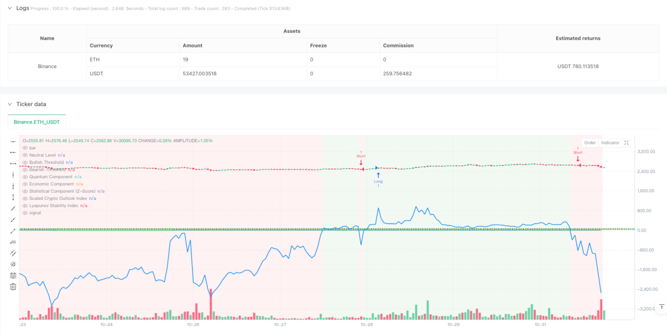
এই কৌশলটি একটি উদ্ভাবনী পরিমাণযুক্ত ট্রেডিং সিস্টেম যা কোয়ান্টাম মেকানিক্স, পরিসংখ্যান এবং অর্থনীতির নীতিগুলিকে একত্রিত করে। এটি একটি সহজ মুভিং এভারেজ (এসএমএ), জেড-স্কোর পরিসংখ্যানগত বিশ্লেষণ, কোয়ান্টাম অস্থিরতা উপাদান, অর্থনৈতিক গতিশীলতা সূচক এবং লিয়াপনোভ স্থিতিশীলতা সূচককে একত্রিত করে একটি বিস্তৃত বাজার বিশ্লেষণ কাঠামো তৈরি করে। এই কৌশলটির কেন্দ্রবিন্দু হল এই বহুমাত্রিক সূচকগুলির একটি ভারসাম্যযুক্ত সমন্বয়, একটি সমন্বিত বাজার প্রত্যাশা সূচক (সিওআই) তৈরি করা, যা ট্রেডিং সিদ্ধান্তগুলিকে নির্দেশ করে।

কৌশল নীতি

এই কৌশলটি পাঁচটি প্রধান প্রযুক্তিগত স্তম্ভের উপর ভিত্তি করে তৈরি করা হয়েছেঃ

1. পরিসংখ্যান বিশ্লেষণ মডিউল এসএমএ এবং স্ট্যান্ডার্ড ডিফারেনশিয়াল ব্যবহার করে জেড-স্কোর গণনা করে, যা দামের আপেক্ষিক অবস্থান মূল্যায়ন করে।
2. কোয়ান্টাম মডিউলটি Z-Score কে একটি ওসিলারে রূপান্তর করে, যা কোয়ান্টাম রাষ্ট্রের ওল্টার বৈশিষ্ট্যকে সূচক এবং সিন্ডিকেট ফাংশন দ্বারা অনুকরণ করে।
3. ইকোনোমিক কম্পোনেন্ট বাজার গতিশীলতা পরিমাপ করার জন্য দ্রুত এবং ধীর EMA এর অনুপাত ব্যবহার করে।
4. লিয়াপ্নভ সূচকটি বাজারের অবস্থা মূল্যায়ন করে, যা কোয়ান্টাম এবং অর্থনৈতিক উপাদানগুলির সমন্বিত স্থায়িত্ব বিশ্লেষণ করে।
5. সমন্বিত বাজার প্রত্যাশা সূচক (COI) সমস্ত উপাদানকে বিভিন্ন ওজনের সাথে একত্রিত করে চূড়ান্ত লেনদেনের সংকেত গঠন করে।

কৌশলগত সুবিধা

1. মাল্টি-ডাইমেনশনাল বিশ্লেষণ বাজারকে আরও ব্যাপকভাবে উপলব্ধি করে এবং একক সূচক দ্বারা সম্ভাব্য বিভ্রান্তি হ্রাস করে।
2. কোয়ান্টাম কম্পোনেন্টের প্রবর্তনের ফলে বাজারের অনন্য ওঠানামা এবং স্বল্পমেয়াদী সুযোগকে কাজে লাগানো সম্ভব হয়েছে।
3. লিয়াপনভ সূচকের ব্যবহার বাজার স্থিতিশীলতার কার্যকর মূল্যায়ন করে এবং ঝুঁকি ব্যবস্থাপনার দক্ষতা বাড়ায়।
4. ওজন-নির্ধারণযোগ্য নকশাটি বিভিন্ন বাজার পরিস্থিতিতে কৌশলগুলিকে নমনীয়ভাবে মানিয়ে নিতে দেয়।
5. সমন্বিত সূচকের নিরপেক্ষ রেখা নকশা স্পষ্ট ট্রেডিং সিগন্যাল সীমানা প্রদান করে।

কৌশলগত ঝুঁকি

1. একাধিক সূচকগুলি প্রবেশের সময়কে প্রভাবিত করতে পারে, যার ফলে সংকেত বিলম্বিত হতে পারে।
2. প্যারামিটার অপ্টিমাইজেশনের ফলে ওভারফিট হওয়ার ঝুঁকি রয়েছে।
3. উচ্চ অস্থিরতার বাজারে, কোয়ান্টাম উপাদানগুলি খুব ঘন ঘন সংকেত তৈরি করতে পারে।
4. অর্থনৈতিক উপাদানগুলি ভুল সংকেত দিতে পারে।
5. ঝুঁকি নিয়ন্ত্রণের জন্য একটি যুক্তিসঙ্গত স্টপ লস সেটআপ প্রয়োজন।

কৌশল অপ্টিমাইজেশনের দিকনির্দেশনা

1. একটি স্বনির্ধারিত ওজন ব্যবস্থা চালু করা, বাজারের গতিশীলতার উপর ভিত্তি করে উপাদানগুলির ওজনকে সামঞ্জস্য করা।
2. উচ্চতর তরঙ্গের সময় সংকেত সংবেদনশীলতা সামঞ্জস্য করার জন্য তরঙ্গ হার ফিল্টার বাড়ান।
3. মার্কেট সেন্টিমেন্ট ইন্ডিকেটরগুলিকে সংহত করে, যা অতিরিক্ত নিশ্চিতকরণ সংকেত প্রদান করে।
4. বাজারের অবস্থার উপর ভিত্তি করে স্টপ লেভেলের পরিবর্তনশীল স্টপ মেকানিজম তৈরি করা।
5. সময় ফিল্টার যুক্ত করুন, যাতে অকার্যকর ট্রেডিংয়ের সময় পজিশন করা থেকে বিরত থাকুন।

সারসংক্ষেপ

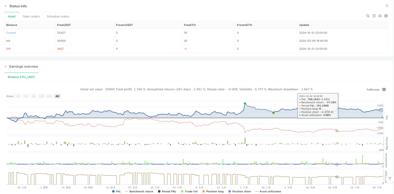
এটি একটি উদ্ভাবনী পরিমাণগত ট্রেডিং কৌশল যা বহু-বিষয়ক তত্ত্বকে একত্রিত করে একটি বিস্তৃত বাজার বিশ্লেষণ কাঠামো তৈরি করে। যদিও কিছু জায়গায় অপ্টিমাইজেশনের প্রয়োজন রয়েছে, তবে এর বহু-মাত্রিক বিশ্লেষণ পদ্ধতিটি ট্রেডিং সিদ্ধান্তের জন্য একটি অনন্য দৃষ্টিভঙ্গি সরবরাহ করে। ক্রমাগত অপ্টিমাইজেশন এবং ঝুঁকি পরিচালনার উন্নতির মাধ্যমে, কৌশলটি বিভিন্ন বাজারের পরিবেশে স্থিতিশীল পারফরম্যান্স বজায় রাখার প্রত্যাশা করে।