Multi-Timeline-Trendfolgestrategie

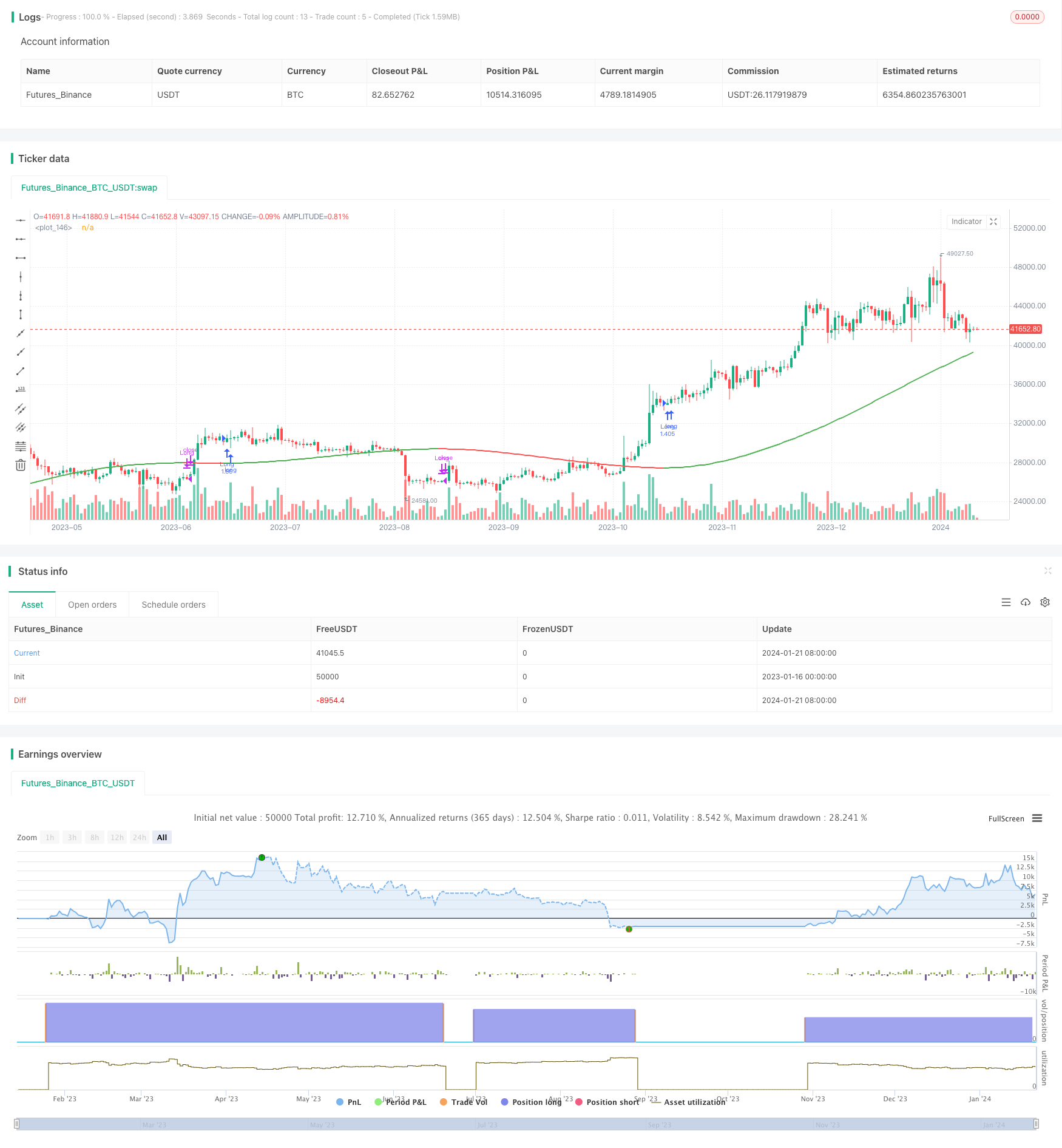
/*backtest
start: 2023-01-16 00:00:00
end: 2024-01-22 00:00:00
period: 1d
basePeriod: 1h
exchanges: [{"eid":"Futures_Binance","currency":"BTC_USDT"}]
*/

// This source code is subject to the terms of the Mozilla Public License 2.0 at https://mozilla.org/MPL/2.0/
// @version=5
// Author = TradeAutomation


strategy(title="Multi MA Trend Following Strategy Template", shorttitle="Multi Trend", process_orders_on_close=true, overlay=true, commission_type=strategy.commission.cash_per_order, commission_value=1, slippage = 0, margin_short = 75, margin_long = 75, initial_capital = 100000000, default_qty_type=strategy.percent_of_equity, default_qty_value=100)

// Backtest Date Range Inputs // 
StartTime = input(defval=timestamp('01 Jan 2019 05:00 +0000'), group="Date Rangte", title='Start Time')
EndTime = input(defval=timestamp('01 Jan 2099 00:00 +0000'), group="Date Range", title='End Time')
InDateRange = true

// Trend Selector //
TrendSelectorInput = input.string(title="Trend Selector", defval="JMA", group="Core Settings", options=["ALMA", "DEMA", "EMA", "HMA", "JMA", "KAMA", "Linear Regression (LSMA)", "RMA", "SMA", "SMMA", "Source", "SuperTrend", "TEMA", "TMA", "VAMA", "VIDYA", "VMA", "VWMA", "WMA", "WWMA", "ZLEMA"], tooltip="Select your moving average")
src = input.source(close, "Source", group="Core Settings", tooltip="This is the price source being used for the moving averages to calculate based on")
length = input.int(200, "MA Length", group="Core Settings", tooltip="This is the amount of historical bars being used for the moving averages to calculate based on")
LineWidth = input.int(2, "Line Width", group="Core Settings", tooltip="This is the width of the line plotted that represents the selected trend")

// Individual Moving Average / Regression Setting //
AlmaOffset = input.float(0.85, "ALMA Offset", group="Individual MA Settings", tooltip="This only applies when ALMA is selected")
AlmaSigma = input.float(6, "ALMA Sigma", group="Individual MA Settings", tooltip="This only applies when ALMA is selected")
ATRFactor = input.float(3, "ATR Multiplier For SuperTrend", group="Individual MA Settings", tooltip="This only applies when SuperTrend is selected")
ATRLength = input.int(12, "ATR Length For SuperTrend", group="Individual MA Settings", tooltip="This only applies when SuperTrend is selected")
JMApower = input.int(2, "JMA Power Parameter", group="Individual MA Settings", tooltip="This only applies when JMA is selected")
KamaAlpha = input.float(3, "KAMA's Alpha", minval=1,step=0.5, group="Individual MA Settings", tooltip="This only applies when KAMA is selected")
LinRegOffset = input.int(0, "Linear Regression Offset", group="Individual MA Settings", tooltip="This only applies when Linear Regression is selected")
VAMALookback =input.int(12, "VAMA Volatility lookback", group="Individual MA Settings", tooltip="This only applies when VAMA is selected")

// Trend Indicators in Library //
ALMA = ta.alma(src, length, AlmaOffset, AlmaSigma) 
EMA = ta.ema(src, length)
HMA = ta.hma(src, length)
LinReg = ta.linreg(src, length, LinRegOffset)
RMA = ta.rma(src, length)
SMA = ta.sma(src, length)
VWMA = ta.vwma(src, length)
WMA = ta.wma(src, length)

// Additional Trend Indicators Written and/or Open Sourced //
//DEMA
de1 = ta.ema(src, length)
de2 = ta.ema(de1, length)
DEMA = 2 * de1 - de2

//JMA [Capissmo]
beta = 0.45*(length-1)/(0.45*(length-1)+2)
alpha = math.pow(beta, JMApower)
L0=0.0, L1=0.0, L2=0.0, L3=0.0, JMA=0.0
L0 := (1-alpha)*src + alpha*nz(L0[1])
L1 := (src - L0[0])*(1-beta) + beta*nz(L1[1])
L2 := L0[0] + L1[0]
L3 := (L2[0] - nz(JMA[1]))*((1-alpha)*(1-alpha)) + (alpha*alpha)*nz(L3[1])
JMA := nz(JMA[1]) + L3[0]

//KAMA
var KAMA = 0.0
fastAlpha = 2.0 / (KamaAlpha + 1)
slowAlpha = 2.0 / 31
momentum = math.abs(ta.change(src, length))
volatility = math.sum(math.abs(ta.change(src)), length)
efficiencyRatio = volatility != 0 ? momentum / volatility : 0
smoothingConstant = math.pow((efficiencyRatio * (fastAlpha - slowAlpha)) + slowAlpha, 2)
KAMA := nz(KAMA[1], src) + smoothingConstant * (src - nz(KAMA[1], src))

//SMMA
var SMMA = 0.0
SMMA := na(SMMA[1]) ? ta.sma(src, length) : (SMMA[1] * (length - 1) + src) / length

//SuperTrend
ATR = ta.atr(ATRLength)
Signal = ATRFactor*ATR
var SuperTrend = 0.0
SuperTrend := if src>SuperTrend[1] and src[1]>SuperTrend[1]
    math.max(SuperTrend[1], src-Signal)
else if src<SuperTrend[1] and src[1]<SuperTrend[1]
    math.min(SuperTrend[1], src+Signal)
else if src>SuperTrend[1]
    src-Signal 
else 
    src+Signal

//TEMA
t1 = ta.ema(src, length)
t2 = ta.ema(t1, length)
t3 = ta.ema(t2, length)
TEMA = 3 * (t1 - t2) + t3

//TMA
TMA = ta.sma(ta.sma(src, math.ceil(length / 2)), math.floor(length / 2) + 1)

//VAMA
mid=ta.ema(src,length)
dev=src-mid
vol_up=ta.highest(dev,VAMALookback)
vol_down=ta.lowest(dev,VAMALookback)
VAMA = mid+math.avg(vol_up,vol_down)

//VIDYA [KivancOzbilgic]
var VIDYA=0.0
VMAalpha=2/(length+1)
ud1=src>src[1] ? src-src[1] : 0
dd1=src<src[1] ? src[1]-src : 0
UD=math.sum(ud1,9)
DD=math.sum(dd1,9)
CMO=nz((UD-DD)/(UD+DD))
VIDYA := na(VIDYA[1]) ? ta.sma(src, length) : nz(VMAalpha*math.abs(CMO)*src)+(1-VMAalpha*math.abs(CMO))*nz(VIDYA[1])

//VMA [LazyBear]
sc = 1/length
pdm = math.max((src - src[1]), 0)
mdm = math.max((src[1] - src), 0)
var pdmS = 0.0
var mdmS = 0.0
pdmS := ((1 - sc)*nz(pdmS[1]) + sc*pdm)
mdmS := ((1 - sc)*nz(mdmS[1]) + sc*mdm)
s = pdmS + mdmS
pdi = pdmS/s
mdi = mdmS/s
var pdiS = 0.0
var mdiS = 0.0
pdiS := ((1 - sc)*nz(pdiS[1]) + sc*pdi)
mdiS := ((1 - sc)*nz(mdiS[1]) + sc*mdi)
d = math.abs(pdiS - mdiS)
s1 = pdiS + mdiS
var iS = 0.0
iS := ((1 - sc)*nz(iS[1]) + sc*d/s1)
hhv = ta.highest(iS, length) 
llv = ta.lowest(iS, length) 
d1 = hhv - llv
vi = (iS - llv)/d1
var VMA=0.0
VMA := sc*vi*src + (1 - sc*vi)*nz(VMA[1])

//WWMA
var WWMA=0.0
WWMA := (1/length)*src + (1-(1/length))*nz(WWMA[1])

//Zero Lag EMA
EMA1 = ta.ema(src,length)
EMA2 = ta.ema(EMA1,length)
Diff = EMA1 - EMA2
ZLEMA = EMA1 + Diff

// Trend Mapping and Plotting //
Trend = TrendSelectorInput == "ALMA" ? ALMA : TrendSelectorInput == "DEMA" ? DEMA : TrendSelectorInput == "EMA" ? EMA : TrendSelectorInput == "HMA" ? HMA : TrendSelectorInput == "JMA" ? JMA : TrendSelectorInput == "KAMA" ? KAMA : TrendSelectorInput == "Linear Regression (LSMA)" ? LinReg : TrendSelectorInput == "RMA" ? RMA : TrendSelectorInput == "SMA" ? SMA : TrendSelectorInput == "SMMA" ? SMMA : TrendSelectorInput == "Source" ? src : TrendSelectorInput == "SuperTrend" ? SuperTrend : TrendSelectorInput == "TEMA" ? TEMA : TrendSelectorInput == "TMA" ? TMA : TrendSelectorInput == "VAMA" ? VAMA : TrendSelectorInput == "VIDYA" ? VIDYA : TrendSelectorInput == "VMA" ? VMA : TrendSelectorInput == "VWMA" ? VWMA : TrendSelectorInput == "WMA" ? WMA : TrendSelectorInput == "WWMA" ? WWMA : TrendSelectorInput == "ZLEMA" ? ZLEMA : SMA
plot(Trend, color=(Trend>Trend[1]) ? color.green : (Trend<Trend[1]) ? color.red : (Trend==Trend[1]) ? color.gray : color.black, linewidth=LineWidth)

// Entry & Exit Functions //

if (InDateRange)
    strategy.entry("Long", strategy.long, when = ta.crossover(Trend, Trend[1]))
    strategy.close("Long", when = ta.crossunder(Trend, Trend[1]))
if (not InDateRange)
    strategy.close_all()