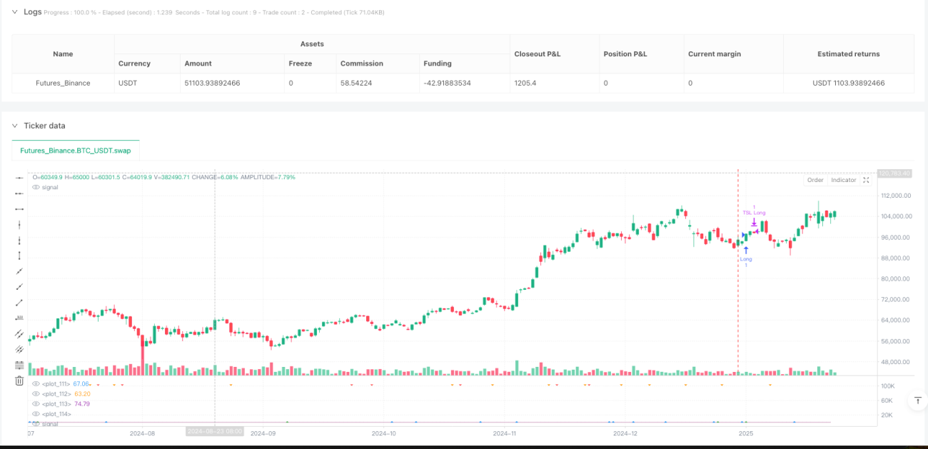
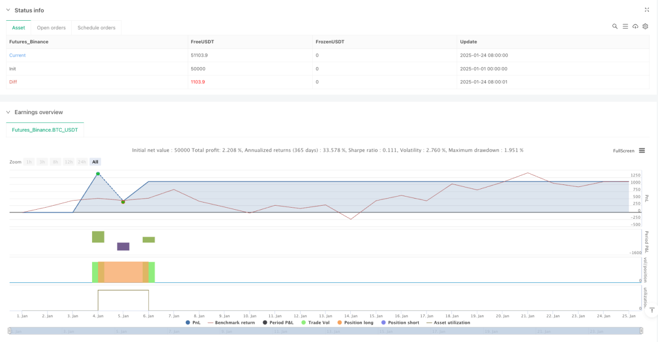
Adaptive dynamische KDJ-Indikatorstrategie mit mehreren Zeitrahmen

/*backtest
start: 2025-01-01 00:00:00
end: 2025-01-25 00:00:00
period: 1d
basePeriod: 1d
exchanges: [{"eid":"Futures_Binance","currency":"BTC_USDT"}]
*/

// This Pine Script™ is subject to the Mozilla Public License 2.0 (https://mozilla.org/MPL/2.0/)
// © Lausekopf

//@version=5
strategy("Adaptive KDJ (MTF)", overlay=false)

// Dropdown for the swing length calculation method
method = input.int(1, title="Calculation Method", options=[1, 2, 3], tooltip="1: Volatility Based\n2: Inverse Volatility\n3: Fixed Length")

// Fixed length for method 3
fixedLength = input.int(9, title="Fixed KDJ Length", minval=3, maxval=15)

// Timeframes
tf1 = input.timeframe("1", title="Timeframe 1")
tf2 = input.timeframe("5", title="Timeframe 2")
tf3 = input.timeframe("15", title="Timeframe 3")

// Timeframe weighting
weightOption = input.int(1, title="Timeframe Weighting", options=[1, 2, 3, 4, 5])
weightTF1 = weightOption == 1 ? 0.5 : weightOption == 2 ? 0.4 : weightOption == 3 ? 0.33 : weightOption == 4 ? 0.2 : 0.1
weightTF2 = 0.33
weightTF3 = 1.0 - (weightTF1 + weightTF2)

// EMA smoothing length
smoothingLength = input.int(5, title="EMA Smoothing Length", minval=1, maxval=50)

// Trend calculation period
trendLength = input.int(40, title="Trend Calculation Period", minval=5, maxval=50)

// KDJ function
f_kdj(len, srcHigh, srcLow, srcClose) =>
    roundedLen = int(math.round(len))
    high_max = ta.highest(srcHigh, roundedLen)
    low_min = ta.lowest(srcLow, roundedLen)
    rsv = 100 * (srcClose - low_min) / (high_max - low_min)
    k = ta.sma(rsv, 3)
    d = ta.sma(k, 3)
    j = 3 * k - 2 * d
    [k, d, j]

// Swing length function
f_swingLength(tf) =>
    atrLen = 14
    volatility = request.security(syminfo.tickerid, tf, ta.atr(atrLen) / close)
    var float length = na
    if method == 1
        length := volatility > 0.03 ? 3 : volatility > 0.002 ? 14 : 15
    if method == 2
        length := 18
    if method == 3
        length := fixedLength
    length

// Calculate swing lengths for each timeframe
swingLength1 = f_swingLength(tf1)
swingLength2 = f_swingLength(tf2)
swingLength3 = f_swingLength(tf3)

// Calculate KDJ values
[k1, d1, j1] = f_kdj(swingLength1, request.security(syminfo.tickerid, tf1, high), request.security(syminfo.tickerid, tf1, low), request.security(syminfo.tickerid, tf1, close))
[k2, d2, j2] = f_kdj(swingLength2, request.security(syminfo.tickerid, tf2, high), request.security(syminfo.tickerid, tf2, low), request.security(syminfo.tickerid, tf2, close))
[k3, d3, j3] = f_kdj(swingLength3, request.security(syminfo.tickerid, tf3, high), request.security(syminfo.tickerid, tf3, low), request.security(syminfo.tickerid, tf3, close))

// Weighted averages
avgK = (k1 * weightTF1 + k2 * weightTF2 + k3 * weightTF3)
avgD = (d1 * weightTF1 + d2 * weightTF2 + d3 * weightTF3)
avgJ = (j1 * weightTF1 + j2 * weightTF2 + j3 * weightTF3)
smoothAvgK = ta.ema(avgK, smoothingLength)
smoothAvgD = ta.ema(avgD, smoothingLength)
smoothAvgJ = ta.ema(avgJ, smoothingLength)
smoothAvgTotal = ta.ema((avgK + avgD + avgJ) / 3, smoothingLength)

// Trend determination
trendAvg = ta.sma(smoothAvgTotal, trendLength)
isUptrend = trendAvg > 60
isDowntrend = trendAvg < 40

// Dynamic signal thresholds
buyLevel = isUptrend ? 40 : isDowntrend ? 15 : 25
sellLevel = isUptrend ? 85 : isDowntrend ? 60 : 75

// Buy/Sell signals
buySignal = smoothAvgJ < buyLevel and ta.crossover(smoothAvgK, smoothAvgD)
sellSignal = smoothAvgJ > sellLevel and ta.crossunder(smoothAvgK, smoothAvgD)

// Anticipated signals
anticipateBuy = (smoothAvgK - smoothAvgK[1]) > 0 and (smoothAvgD - smoothAvgD[1]) < 0 and math.abs(smoothAvgK - smoothAvgD) < 5
anticipateSell = (smoothAvgK - smoothAvgK[1]) < 0 and (smoothAvgD - smoothAvgD[1]) > 0 and math.abs(smoothAvgK - smoothAvgD) < 5

// Entry conditions
longEntryCondition = (buySignal or anticipateBuy) and smoothAvgTotal < 22
shortEntryCondition = (sellSignal or anticipateSell) and smoothAvgTotal > 78

// Entry orders
strategy.entry("Long", strategy.long, when=longEntryCondition)
strategy.entry("Short", strategy.short, when=shortEntryCondition)

// Trailing Stop-Loss
atrMultiplierTSL = 2.5
atrValueTSL = ta.atr(12) * atrMultiplierTSL
strategy.exit("TSL Long", from_entry="Long", trail_points=atrValueTSL / syminfo.mintick, stop=open * 0.9972)
strategy.exit("TSL Short", from_entry="Short", trail_points=atrValueTSL / syminfo.mintick, stop=open * 1.0028)

// Plot signals
plotshape(series=buySignal, location=location.bottom, style=shape.triangleup, color=color.green, size=size.small)
plotshape(series=sellSignal, location=location.top, style=shape.triangledown, color=color.red, size=size.small)
plotshape(series=anticipateBuy, location=location.bottom, style=shape.triangleup, color=color.blue, size=size.tiny, offset=-1)
plotshape(series=anticipateSell, location=location.top, style=shape.triangledown, color=color.orange, size=size.tiny, offset=-1)

// Plot KDJ lines
plot(smoothAvgK, color=color.blue, linewidth=1)
plot(smoothAvgD, color=color.orange, linewidth=1)
plot(smoothAvgJ, color=color.purple, linewidth=1)
plot(smoothAvgTotal, color=color.white, linewidth=1)

// Alert for impending signals
alertcondition(anticipateBuy or anticipateSell, title='Impending KDJ Crossover', message='Possible KDJ crossover detected!')
// This Pine Script™ code is subject to the terms of the Mozilla Public License 2.0 at https://mozilla.org/MPL/2.0/
// © Lausekopf