Multi-Kernel Regression Dynamic Trend Trading Strategy

DR MKR ATR SMA MA200 TP SL
Created on: 2025-02-24 09:27:50 Modified on: 2025-02-24 09:27:50
Copy: 0 Number of hits: 805
avatar of ianzeng123 ianzeng123
2
Follow
319
Followers

 Multi-Kernel Regression Dynamic Trend Trading Strategy  Multi-Kernel Regression Dynamic Trend Trading Strategy

Overview

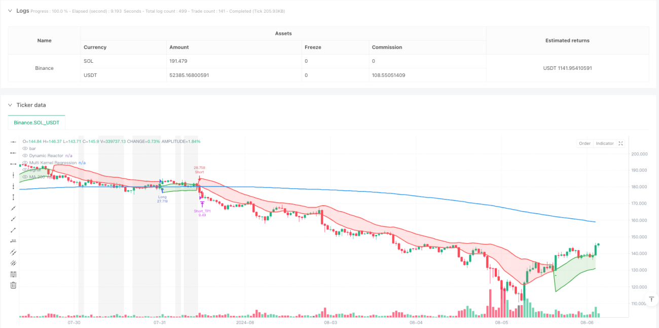
This is a trend following trading strategy that combines Dynamic Reactor (DR) and Multi-Kernel Regression (MKR). The strategy calculates dynamic support/resistance lines using ATR and SMA, and identifies market trends using a combination of Gaussian and Epanechnikov kernel regression. It also incorporates MA200 as a long-term trend filter and implements a triple take-profit and stop-loss mechanism.

Strategy Principles

The strategy consists of four core components: 1. Dynamic Reactor (DR): Uses ATR and SMA to construct dynamic support/resistance bands, determining trend direction based on price position. The lower band serves as support in uptrends, while the upper band acts as resistance in downtrends.

  1. Multi-Kernel Regression (MKR): Combines Gaussian and Epanechnikov kernels for price regression, optimizing the combination through adjustable weight parameters. This method better captures the dynamic characteristics of price movements.

  2. MA200 Trend Filter: Uses the 200-day moving average as a long-term trend indicator, only allowing trades when price and MA200 form clear trends, and identifies consolidation periods through the consolidationRange parameter.

  3. Money Management System: Employs triple take-profit targets (1.5%, 3.0%, 4.5%) and 1% stop-loss, distributing positions in 33%-33%-34% ratio to maximize returns while controlling risk.

Strategy Advantages

  1. Trend Identification Reliability: Dual confirmation through DR and MKR improves trend judgment accuracy.
  2. Risk Management Completeness: Combines segmented profit-taking with unified stop-loss to protect profits and limit losses.
  3. High Adaptability: Multi-kernel regression method better adapts to different market conditions.
  4. Clear Trading Signals: Trend transition points have clear graphical indicators.
  5. Comprehensive Filtering: Excludes unfavorable market environments through MA200 and consolidation period identification.

Strategy Risks

  1. Parameter Optimization Risk: Over-optimization may lead to overfitting, reducing actual strategy performance.
  2. Lag Risk: Moving averages and regression indicators have inherent lag, potentially missing important turning points.
  3. Market Environment Dependency: May underperform in highly volatile or ranging markets.
  4. Execution Risk: Multiple take-profit and stop-loss orders may not execute fully due to liquidity issues.

Strategy Optimization Directions

  1. Dynamic Parameter Adjustment: Automatically adjust ATR multiplier and regression period based on market volatility.
  2. Signal Confirmation Enhancement: Add volume, volatility, and other auxiliary indicators to improve signal reliability.
  3. Position Management Optimization: Implement volatility-based dynamic position management.
  4. Market Environment Classification: Add market state identification module to use different parameter settings in different market environments.

Summary

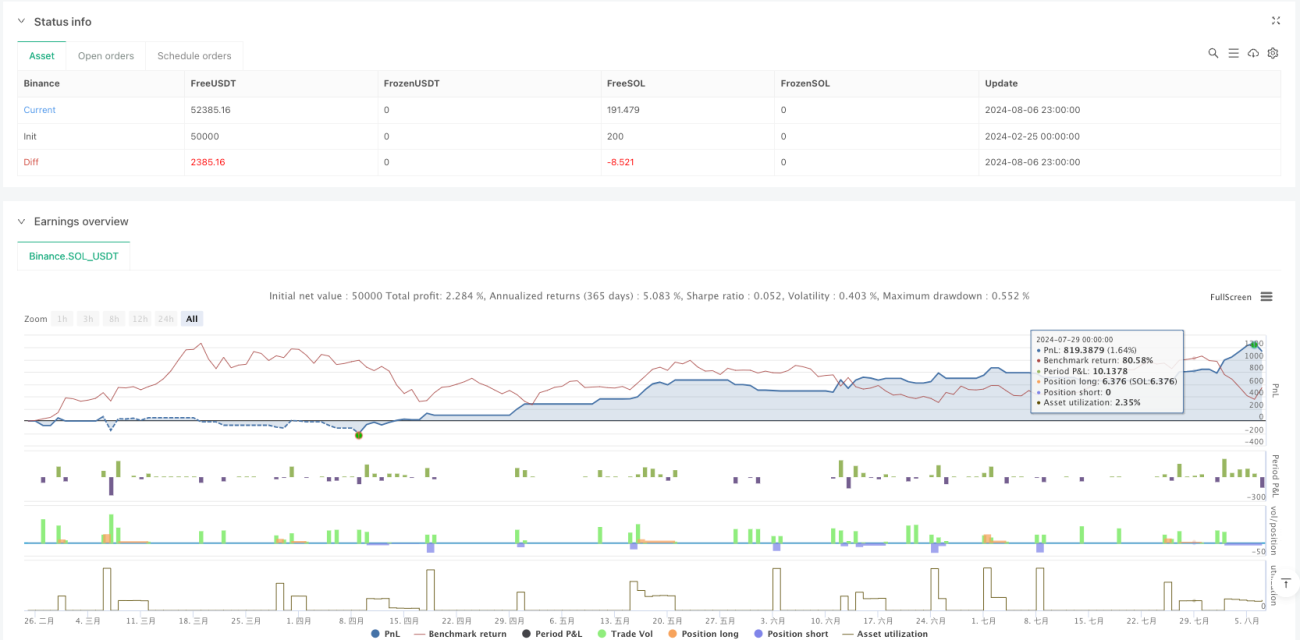
This strategy builds a complete trading system by integrating multiple technical indicators and advanced statistical methods. Its strengths lie in accurate trend capture and comprehensive risk management, but attention must be paid to parameter optimization and market adaptability issues. The strategy has room for further improvement through the suggested optimization directions.

Strategy source code
/*backtest
start: 2024-02-25 00:00:00
end: 2024-08-07 00:00:00
period: 1h
basePeriod: 1h
exchanges: [{"eid":"Binance","currency":"SOL_USDT"}]
*/

//@version=5
strategy("DR + Multi Kernel Regression + Signals + MA200 with TP/SL (Optimized)", overlay=true, shorttitle="DR+MKR+Signals+MA200_TP_SL_Opt", pyramiding=0, default_qty_type=strategy.percent_of_equity, default_qty_value=10)

// =====================================================================
// PARTEA 1: Dynamic Reactor – linie unică colorată în funcție de trend
// =====================================================================
// Parametri pentru Dynamic Reactor
atrLength  = input.int(14, title="Lungimea ATR", minval=1)
smaLength  = input.int(20, title="Lungimea SMA", minval=1)
multiplier = input.float(1.5, title="Multiplicator ATR", minval=0.1, step=0.1)
// Calculăm ATR și SMA
atrValue = ta.atr(atrLength)
smaValue = ta.sma(close, smaLength)
// Benzile de bază
basicUpper = smaValue + atrValue * multiplier
basicLower = smaValue - atrValue * multiplier
// Calculăm benzile finale (similar cu SuperTrend)
var float finalUpper = basicUpper
var float finalLower = basicLower
if bar_index > 0
    finalUpper := close[1] > finalUpper[1] ? math.max(basicUpper, finalUpper[1]) : basicUpper
    finalLower := close[1] < finalLower[1] ? math.min(basicLower, finalLower[1]) : basicLower
// Determinăm trendul curent:
// - Dacă prețul curent este peste finalUpper din bara anterioară → uptrend (1)
// - Dacă prețul este sub finalLower din bara anterioară → downtrend (-1)
// - Altfel, păstrăm trendul precedent.
var int trend = 1
if bar_index > 0
    trend := close > finalUpper[1] ? 1 : close < finalLower[1] ? -1 : nz(trend[1], 1)
// Linia Dynamic Reactor:
// - În uptrend se utilizează finalLower (nivel de suport)
// - În downtrend se utilizează finalUpper (nivel de rezistență)
drLine = trend == 1 ? finalLower : finalUpper
// Plotăm linia Dynamic Reactor
p_dr = plot(drLine, color=trend == 1 ? color.green : color.red, title="Dynamic Reactor", linewidth=2)


// =====================================================================
// PARTEA 2: Multi Kernel Regression
// =====================================================================
// Parametri pentru regresia cu kernel
regLength = input.int(50, title="Perioada regresiei", minval=1)
h1        = input.float(10.0, title="Bandă Gaussiană (h1)", minval=0.1)
h2        = input.float(10.0, title="Bandă Epanechnikov (h2)", minval=0.1)
alpha     = input.float(0.5, title="Pondere Kernel Gaussian (0-1)", minval=0, maxval=1)
// Funcție: regresie cu kernel Gaussian
f_gaussian_regression(bw) =>
    num = 0.0
    den = 0.0
    for i = 0 to regLength - 1
        // Kernel Gaussian: K(x) = exp(-0.5 * (i/bw)^2)
        weight = math.exp(-0.5 * math.pow(i / bw, 2))
        num += close[i] * weight
        den += weight
    num / (den == 0 ? 1 : den)
// Funcție: regresie cu kernel Epanechnikov
f_epanechnikov_regression(bw) =>
    num = 0.0
    den = 0.0
    for i = 0 to regLength - 1
        ratio = i / bw
        // Kernel Epanechnikov: K(u) = 1 - u^2 pentru |u| <= 1, altfel 0
        weight = math.abs(ratio) <= 1 ? (1 - math.pow(ratio, 2)) : 0
        num += close[i] * weight
        den += weight
    num / (den == 0 ? 1 : den)
// Calculăm regresiile pentru fiecare kernel
regGauss = f_gaussian_regression(h1)
regEpan  = f_epanechnikov_regression(h2)
// Combinăm rezultatele celor două regresii
multiKernelRegression = alpha * regGauss + (1 - alpha) * regEpan
// Plotăm linia Multi Kernel Regression
p_mkr = plot(multiKernelRegression, color=trend == 1 ? color.green : color.red, title="Multi Kernel Regression", linewidth=2)

// Adăugăm ceata (fill) între Dynamic Reactor și Multi Kernel Regression
fillColor = trend == 1 ? color.new(color.green, 80) : color.new(color.red, 80)
fill(p_dr, p_mkr, color=fillColor, title="Trend Fill")


// =====================================================================
// PARTEA 2.1: MA 200 și evidențierea consolidării
// =====================================================================
// Calculăm MA 200 pentru trend pe termen lung
ma200 = ta.sma(close, 200)
p_ma200 = plot(ma200, color=color.blue, title="MA 200", linewidth=2)
// Parametru pentru detectarea consolidării (cât de aproape trebuie să fie prețul de MA200, în %)
consolidationRange = input.float(1.0, title="Consolidation Range (%)", minval=0.1, step=0.1)
// Determinăm dacă suntem într-o fază de consolidare (prețul este în interiorul unui interval mic în jurul MA200)
isConsolidation = (math.abs(close - ma200) / ma200 * 100) < consolidationRange
// Colorăm fundalul graficului cu un gri translucid atunci când e consolidare
bgcolor(isConsolidation ? color.new(color.gray, 90) : na, title="Consolidation BG")


// =====================================================================
// PARTEA 3: Semnale Buy și Sell
// =====================================================================
// Semnale de intrare:
// - Buy Signal: când linia Multi Kernel Regression trece peste linia Dynamic Reactor
// - Sell Signal: când linia Multi Kernel Regression trece sub linia Dynamic Reactor
buySignal  = ta.crossover(multiKernelRegression, drLine)
sellSignal = ta.crossunder(multiKernelRegression, drLine)

// Plotăm semnalele pe grafic
plotshape(buySignal, style=shape.triangleup, location=location.belowbar, color=color.green, size=size.tiny, title="Buy Signal")
plotshape(sellSignal, style=shape.triangledown, location=location.abovebar, color=color.red, size=size.tiny, title="Sell Signal")

// Setăm condiții de alertă
alertcondition(buySignal, title="Buy Alert", message="Buy Signal: Kernel is above Dynamic Reactor")
alertcondition(sellSignal, title="Sell Alert", message="Sell Signal: Kernel is below Dynamic Reactor")


// =====================================================================
// PARTEA 4: Trade Management – Intrări, 3 TP și 1 SL
// =====================================================================
// Parametrii pentru TP și SL (valori ajustate pentru un raport risc-recompensă mai favorabil)
tp1Perc = input.float(1.5, title="TP1 (%)", minval=0.1, step=0.1)
tp2Perc = input.float(3.0, title="TP2 (%)", minval=0.1, step=0.1)
tp3Perc = input.float(4.5, title="TP3 (%)", minval=0.1, step=0.1)
slPerc  = input.float(1.0, title="Stop Loss (%)", minval=0.1, step=0.1)

// ---- Intrări de tranzacționare cu filtrare suplimentară pe baza trendului MA200 și consolidării ----
// Pentru poziții long, intrăm doar când prețul este peste MA200 și nu este în consolidare.
// Pentru poziții short, intrăm doar când prețul este sub MA200 și nu este în consolidare.
if (buySignal and close > ma200 and not isConsolidation)
    strategy.entry("Long", strategy.long)

if (sellSignal and close < ma200 and not isConsolidation)
    strategy.entry("Short", strategy.short)

// ---- Gestionarea ordinelor pentru poziții long ----
if (strategy.position_size > 0)
    entryPrice = strategy.position_avg_price
    // Calculăm nivelurile de TP și SL pentru poziția long
    long_sl = entryPrice * (1 - slPerc / 100)
    long_tp1 = entryPrice * (1 + tp1Perc / 100)
    long_tp2 = entryPrice * (1 + tp2Perc / 100)
    long_tp3 = entryPrice * (1 + tp3Perc / 100)
    
    // Plasăm TP-urile (alocări: 33%, 33% și 34%)
    strategy.exit("Long_TP1", from_entry="Long", limit=long_tp1, qty_percent=33, comment="TP1")
    strategy.exit("Long_TP2", from_entry="Long", limit=long_tp2, qty_percent=33, comment="TP2")
    strategy.exit("Long_TP3", from_entry="Long", limit=long_tp3, qty_percent=34, comment="TP3")
    
    // Plasăm ordinul de SL pentru poziția long
    strategy.exit("Long_SL", from_entry="Long", stop=long_sl, comment="SL")

// ---- Gestionarea ordinelor pentru poziții short ----
if (strategy.position_size < 0)
    entryPrice = strategy.position_avg_price
    // Calculăm nivelurile de TP și SL pentru poziția short
    short_sl = entryPrice * (1 + slPerc / 100)
    short_tp1 = entryPrice * (1 - tp1Perc / 100)
    short_tp2 = entryPrice * (1 - tp2Perc / 100)
    short_tp3 = entryPrice * (1 - tp3Perc / 100)
    
    // Plasăm TP-urile (alocări: 33%, 33% și 34%)
    strategy.exit("Short_TP1", from_entry="Short", limit=short_tp1, qty_percent=33, comment="TP1")
    strategy.exit("Short_TP2", from_entry="Short", limit=short_tp2, qty_percent=33, comment="TP2")
    strategy.exit("Short_TP3", from_entry="Short", limit=short_tp3, qty_percent=34, comment="TP3")
    
    // Plasăm ordinul de SL pentru poziția short
    strategy.exit("Short_SL", from_entry="Short", stop=short_sl, comment="SL")