Pivot Point Detection with Bollinger Band Oscillation Strategy

Overview

The Pivot Point Detection with Bollinger Band Oscillation Strategy is a technical analysis-based trading approach designed to identify key price levels in sideways market movements. The core of this strategy lies in combining Bollinger Band width, Average True Range (ATR), and price position relative to the Bollinger Band middle line to precisely capture trading opportunities in low-volatility environments. By setting specific percentile thresholds, the strategy can filter out periods when market volatility narrows and prices tend to stabilize, thereby predicting potential price breakout directions.

Strategy Principles

The theoretical foundation of this strategy is that markets often experience directional breakouts after periods of low volatility. The specific implementation mechanisms are as follows:

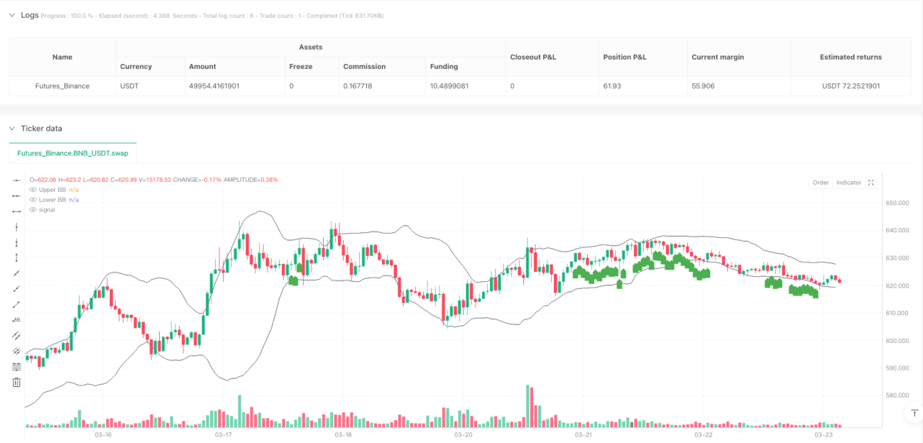
1. Bollinger Bands Calculation: The strategy uses 20 days of price data to calculate a Simple Moving Average (SMA) and standard deviation, then constructs a Bollinger Band channel with a standard deviation factor of 2. Bollinger Band width is defined as (upper band - lower band)/middle band, used to measure market volatility.

2. ATR Normalization Processing: A 14-day Average True Range (ATR) is used and normalized by the current closing price to obtain a relative volatility indicator.

3. Percentile Threshold Filtering: The strategy innovatively applies the concept of percentile thresholds. By calculating the highest and lowest values of Bollinger Band width and normalized ATR within the observation period, then interpolating based on user-defined percentiles (25% and 30%) to determine specific thresholds.

4. Sideways Market Confirmation: When the Bollinger Band width is below the calculated threshold, the market is considered to be in a sideways state.

5. Trade Signal Generation: A buy signal is generated when three conditions are met: the market is in a sideways state, the normalized ATR is below the threshold, and the price is close to the Bollinger Band middle line (deviation not exceeding 2%).

Strategy Advantages

1. Low Risk, High Precision: The strategy focuses on trading opportunities in low-volatility environments, avoiding risks associated with large fluctuations. The combined use of Bollinger Bands and ATR enhances signal reliability.

2. Quantitative Filtering Mechanism: Using a dynamic adjustment mechanism of percentile thresholds, the strategy can adapt to the volatility characteristics of different market environments and instruments, avoiding the limitations that fixed parameters might bring.

3. Strong Adaptability: By calculating relative Bollinger Band width and normalized ATR, the strategy can maintain consistent performance across different price ranges and volatility environments.

4. Easy to Understand and Optimize: The strategy logic is clear, with relatively simple parameters, making it easy to understand and specifically optimize. The strategy uses standard technical indicators without complex mathematical calculations, making it easy for traders to master.

5. Middle Line Trading Advantage: By requiring prices to be close to the Bollinger Band middle line, the strategy effectively avoids the risk of entering at extreme price levels, improving the win rate.

Strategy Risks

1. False Breakout Risk: In low-volatility markets, there may be brief price movements that trigger signals but subsequently retrace, causing false breakouts. This can be mitigated by adding confirmation mechanisms or extending observation time.

2. Parameter Sensitivity: Strategy performance is highly dependent on the settings of Bollinger Band period, standard deviation factor, and percentile thresholds. Different market environments may require different parameter combinations, necessitating regular backtesting and optimization.

3. Market Environment Dependency: This strategy performs excellently in oscillating markets but may miss major trends in strong trending markets or generate too many signals. It is recommended to use it in combination with trend identification indicators.

4. Lack of Stop-Loss Mechanism: There is no explicit stop-loss mechanism in the current code, which needs to be supplemented and improved in actual trading to control single trade risk.

5. Signal Scarcity: Due to relatively stringent conditions, the strategy may not generate trading signals for extended periods, affecting capital utilization efficiency. Consider appropriately relaxing conditions or adding other trading logics.

Strategy Optimization Directions

1. Add Trend Filters: Introduce trend judgment indicators (such as moving average direction, ADX, etc.) to add judgment of the overall market environment while maintaining the original oscillation logic, avoiding counter-trend operations in strong trending markets.

2. Optimize Exit Logic: The current strategy only has entry signals and lacks a clear exit mechanism. Add stop-profit and stop-loss plans based on Bollinger Band boundaries, ATR multiples, or fixed profit-loss ratios to complete the trading loop.

3. Add Volume Confirmation: Trading volume is often an important verification indicator for the validity of price breakouts. Add volume anomaly detection logic to improve signal quality.

4. Optimize Signal Frequency: Balance the relationship between signal frequency and quality by adjusting parameters or adding auxiliary judgment conditions to improve capital utilization efficiency.

5. Add Reverse Signals: Based on similar logic, add conditions for generating short signals to make the strategy more comprehensive and adaptable to more market environments.

6. Parameter Adaptive Mechanism: Introduce a parameter dynamic optimization mechanism to automatically adjust Bollinger Band period and standard deviation factor based on recent market performance to adapt to changing market environments.

Summary

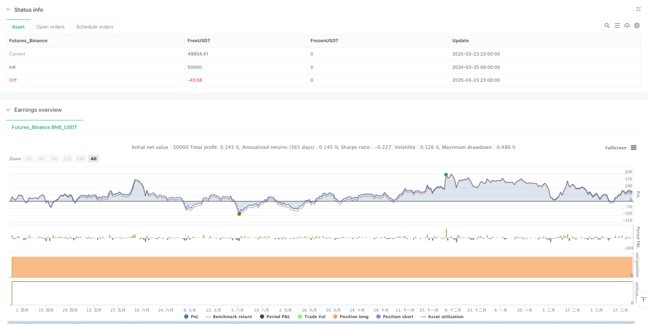
The Pivot Point Detection with Bollinger Band Oscillation Strategy is a quantitative trading method focused on capturing breakthrough opportunities in low-volatility markets. Through the clever combination of Bollinger Band width and normalized ATR, this strategy can effectively identify potential turning points in sideways markets. The core advantages of the strategy lie in its low risk, high adaptability, and clear signal generation logic, particularly suitable for low-volatility market environments. Although there are risks such as parameter sensitivity and signal scarcity, the strategy’s stability and profitability can be further enhanced by introducing trend filtering, optimizing exit logic, and adding volume confirmation. For investors seeking low-risk trading opportunities, this is a strategy worth considering. This strategy is not only applicable for short-term trading but can also be applied to medium and long-term investment decisions by adjusting parameters, demonstrating the application value of technical analysis across different time frames.