
Overview
The Multi-Timeframe RSI-SMA Dynamic Crossover Adaptive Trading System is an advanced quantitative trading strategy that combines Relative Strength Index (RSI) and Simple Moving Average (SMA) crossover signals. What makes this strategy unique is its ability to automatically adjust indicator parameters, risk levels, and filtering conditions according to different timeframes (from 1-minute to monthly charts), achieving cross-timeframe trading adaptability. Through in-depth analysis of the Pine Script code, it's evident that the strategy employs an intelligent parameter adjustment mechanism that automatically optimizes RSI periods, SMA periods, ATR multipliers, take-profit percentages, and volume requirements across different timeframes, thereby maintaining consistent performance in short-term, medium-term, and long-term trading.
Strategy Principle
The core principle of this strategy is based on the crossover signals between RSI and its SMA line, combined with multiple confirmation filters and a dynamic risk management system. The specific operating principles are as follows:
-
Intelligent Parameter Adaptation: The strategy detects the current chart timeframe using the
timeframe.periodfunction, then assigns optimal parameters for various indicators using a switch structure. For example, the RSI period expands from 10 periods on 1-minute charts to 28 periods on monthly charts; SMA periods range from 20 to 200; ATR multipliers increase from 1.5x to 4.5x; take-profit targets range from 3% to 10%. -
Dynamic Indicator Calculation:
- Adaptive RSI-SMA: Calculates RSI values and RSI SMA lines using optimized periods
- Smart Volume Filtering: Adjusts volume requirements based on timeframe, requiring 2x the 20-period average volume for 1-minute charts, but only 0.5x for monthly charts
- Trend Confirmation: Uses crossovers between fast and slow EMAs to confirm uptrends, ensuring trades follow the trend
-
Entry Conditions:
- RSI crosses above its SMA line
- Volume exceeds the dynamic threshold
- Confirmed uptrend (Fast EMA > Slow EMA)
- Closing price greater than opening price (bullish candle)
- Closing price breaks above the 5-period high
-
Exit Conditions:
- RSI crosses below its SMA line
- Price drops below the 5-period low
-
Risk Management:
- Dynamic Stop-Loss: Based on ATR multipliers (from 1.5x to 4.5x), adapting to the volatility characteristics of different timeframes
- Dynamic Take-Profit: Sets percentage targets from 3% to 10% based on entry point, expanding with the timeframe
Strategy Advantages
Through in-depth analysis of the code structure, this strategy demonstrates the following significant advantages:
-
Full Timeframe Adaptability: The most prominent advantage is the strategy's ability to work adaptively across all timeframes from 1-minute to monthly charts without manual intervention to adjust parameters. This solves the common problem of traditional strategies performing inconsistently across different timeframes.
-
Multiple Filtering Mechanisms: The strategy relies not only on RSI-SMA crossover signals but also combines price breakouts, trend confirmation, volume verification, and other multiple filtering conditions, significantly reducing false signals.
-
Dynamic Risk Management: Stop-loss and take-profit levels automatically adjust with timeframe and market volatility. Higher timeframes set wider stop-losses and larger profit targets, which aligns with volatility patterns.
-
Automatic Visualization: The code includes clear visualization elements, including buy markers, stop-loss lines, and take-profit lines, helping traders intuitively understand the trading logic.
-
Low Code Complexity: Despite being powerful, the code structure is clear, well-organized, and logically concise, making it easy to maintain and further optimize.
Strategy Risks
Despite its sophisticated design, the strategy still has the following potential risks:
-
Parameter Optimization Overfitting Risk: Although the strategy sets optimized parameters for different timeframes, these parameters may be derived from historical data optimization, presenting an overfitting risk. The solution is to backtest and validate across multiple market cycles (bull, bear, ranging markets) and different instruments.
-
Rapid Trend Reversal Risk: In highly volatile markets, prices may quickly reverse after triggering an entry signal, causing stop-losses to be hit. It's advisable to pause the strategy during extreme market volatility periods (such as before and after major economic announcements) or add additional filtering conditions.
-
Volume Anomaly Risk: The strategy relies on volume as a filtering condition, but under certain market conditions (such as liquidity droughts), abnormal volume fluctuations may occur, affecting signal quality. Consider adding relative volume indicators or volume accumulation/distribution analysis to enhance filtering effectiveness.
-
Fixed Percentage Take-Profit Limitations: Using fixed percentage take-profits may exit strong trends too early, missing out on larger profits. Consider implementing scaled profit-taking or dynamically adjusting take-profit levels based on trend strength.
-
Timeframe Switching Confusion: Switching timeframes during strategy operation may cause parameter mutations, affecting risk management settings for current positions. It's recommended to close all positions before switching timeframes.
Strategy Optimization Directions
Based on code analysis, the strategy can be optimized in the following aspects:
-
Add Adaptive Momentum Indicators: Incorporate momentum indicators like MACD or OBV as additional confirmation alongside the RSI-SMA system, especially in long-term trading, to improve signal quality. The rationale for this optimization is that momentum indicators better capture trend continuity and strength.
-
Market State Classification Mechanism: Introduce an automatic classification mechanism for market states (range-bound/trending), automatically adjusting strategy preferences based on volatility and directional parameters. This can reduce trading frequency in range-bound markets and increase holding time in trending markets.
-
Dynamic Stop-Loss Optimization: Current stop-losses are based on fixed ATR multipliers. Consider dynamically adjusting stop-losses by incorporating support levels, resistance levels, or key price levels to increase the market relevance of stop-loss settings.
-
Intraday Time Filtering: For short timeframes (1-minute to 1-hour), add intraday time filtering to avoid high volatility periods 30 minutes before market open and close, or focus on specific high-efficiency trading sessions.
-
Machine Learning Parameter Optimization: Introduce simple machine learning algorithms to dynamically optimize RSI and SMA periods, automatically adjusting parameters based on recent market conditions, rather than using preset fixed parameter mappings.
-
Multi-Indicator Resonance System: Expand to a multi-indicator resonance system, combining price action, volume distribution, and market structure analysis to improve signal reliability and anti-interference capabilities.
Summary
The Multi-Timeframe RSI-SMA Dynamic Crossover Adaptive Trading System is an intricately designed quantitative trading strategy. Its most significant feature is the ability to automatically adapt to any timeframe from 1-minute to monthly charts without manual parameter adjustments. The strategy uses RSI crossing above its SMA line as the core signal, combined with multiple filtering conditions and dynamic risk management, achieving cross-timeframe trading adaptability.
This strategy is particularly suitable for traders who need to flexibly switch between multiple timeframes, as well as quantitative analysts who want to build consistent trading systems from short-term to long-term. Through intelligent parameter adjustment, dynamic indicator calculation, and strict entry conditions, the strategy can maintain stable performance across different market environments.
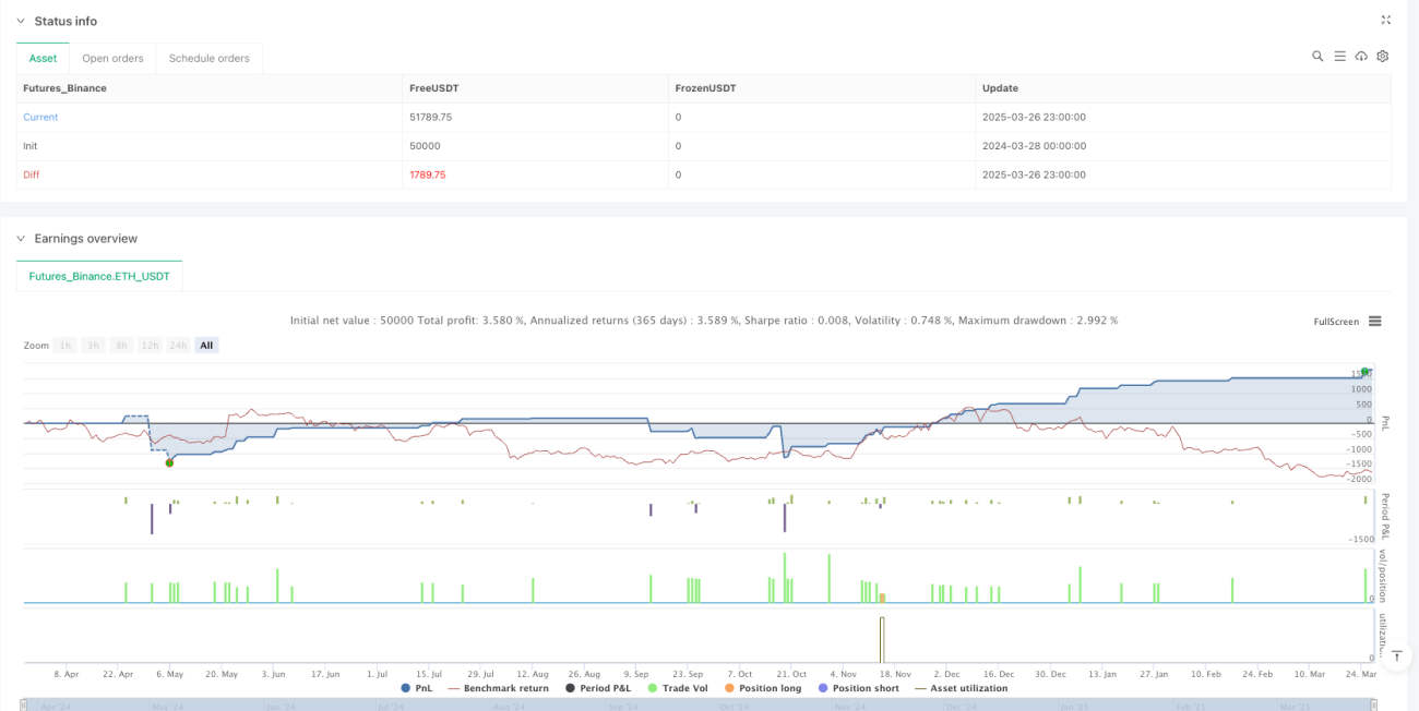
Although risks such as parameter optimization overfitting and rapid trend reversals exist, through the optimization directions proposed in this article, such as adding adaptive momentum indicators, market state classification mechanisms, and machine learning parameter optimization, the strategy's robustness and profitability can be further enhanced. In practical application, it is recommended to conduct thorough backtesting across multiple market cycles and different instruments, combined with 0.1% transaction cost simulation, to verify the strategy's performance in real market environments.
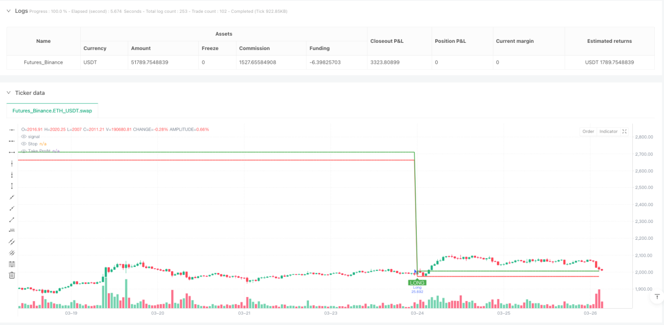
/*backtest
start: 2024-03-28 00:00:00
end: 2025-03-27 00:00:00
period: 1h
basePeriod: 1h
exchanges: [{"eid":"Futures_Binance","currency":"ETH_USDT"}]
*/

//@version=5
strategy("Multi-Timeframe RSI-SMA Strategy [EB]", overlay=true, precision=2, initial_capital=10000, default_qty_type=strategy.percent_of_equity, default_qty_value=100)

//▄▄▄▄▄▄▄▄▄▄▄▄▄▄▄▄▄▄▄▄▄▄▄▄▄▄▄▄▄▄▄▄▄▄▄▄▄▄▄▄▄- 1