
Overview
The Multi-Level Grid Dynamic Equilibrium Trading Strategy is a quantitative trading method based on oscillating ranges, achieving dynamic capital allocation and risk diversification by establishing multi-level grid trading points within preset price ranges. This strategy combines grid trading, Dollar Cost Averaging (DCA), and dynamic take-profit and stop-loss mechanisms, aiming to capture stable returns from market range-bound oscillations. The core concept involves gradually building positions during price declines and systematically taking profits during uptrends, achieving a balance between risk and return through multi-level grid deployment.
Strategy Principles
The core principle of this strategy is based on the assumption that market prices oscillate within specific ranges. First, the strategy establishes a price channel with upper and lower boundaries, determining the oscillation range through user-defined parameters. Within this range, the system calculates multiple equidistant price levels based on grid spacing percentages, forming a grid trading matrix.
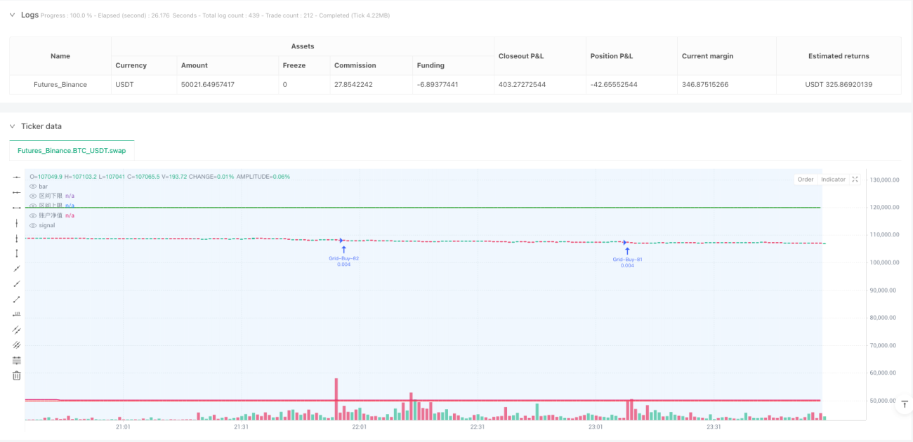
When prices enter the oscillation range without existing positions, the strategy initiates building at the current grid position. Subsequently, when prices move to new grid positions, the system adds to positions according to the set addition ratio, achieving a gradual position-building effect. Each grid position records corresponding entry prices and quantities, providing the basis for subsequent profit-taking operations.
The profit-taking mechanism employs layered processing, where each grid position has independent profit targets. When market prices reach the profit-taking price of a specific grid position, the system closes the corresponding position while maintaining other grid positions. This mechanism ensures the strategy can gradually profit during market uptrends while maintaining certain market exposure.
The strategy also integrates multiple stop-loss protection mechanisms, including both capital-based and price-based stop-losses. Capital stop-loss is based on total account equity drawdown, while price stop-loss is based on the decline from average holding cost. When prices break through preset channels, the strategy immediately closes all positions, avoiding significant losses in trending markets.
Strategy Advantages
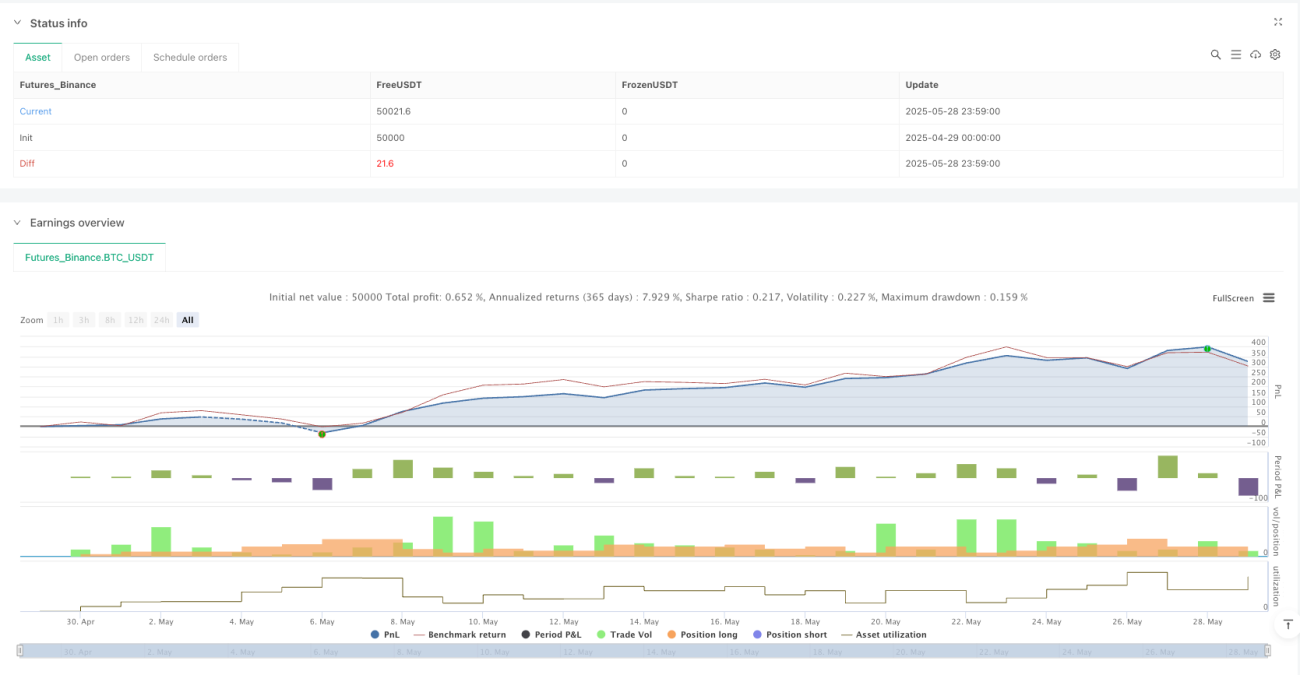
The Multi-Level Grid Dynamic Equilibrium Trading Strategy offers significant risk diversification advantages. By establishing multiple trading positions at different price levels, the strategy effectively reduces timing risks associated with single-point entries. Even if initial entry timing is poor, subsequent gradual position additions can average down costs and improve overall position profitability.
The strategy's high degree of automation reduces subjective and emotional influences in manual decision-making. All trading decisions are based on preset mathematical models and logical rules, ensuring execution consistency and discipline. This mechanized trading approach is particularly suitable for oscillating market environments, continuously capturing arbitrage opportunities from price fluctuations.
Capital utilization efficiency represents another important advantage of this strategy. Through layered position building and layered profit-taking mechanisms, the strategy can flexibly adjust capital allocation under different market conditions. During price decline phases, position sizes gradually increase; during price rise phases, profits are systematically realized. This dynamic balance mechanism helps maximize capital utilization efficiency.
The strategy's risk control mechanisms are comprehensive, incorporating multiple layers of protective measures. Beyond traditional stop-loss mechanisms, the strategy includes channel breakout protection, enabling timely exits when markets experience trending changes, avoiding continued losses in unfavorable market environments.
Strategy Risks
The strategy's primary risk stems from trending market changes. When markets experience unidirectional rallies or declines, grid trading advantages become disadvantages. In unidirectional decline scenarios, the strategy continues adding positions, causing floating losses to expand continuously; in unidirectional rally scenarios, the strategy closes positions prematurely, missing significant upward opportunities.
The reasonableness of range settings directly impacts strategy performance. If oscillation ranges are too narrow, the strategy may frequently trigger channel breakout exits, leading to excessive trading costs; if ranges are too wide, the strategy may fail to trigger profit-taking conditions for extended periods, resulting in low capital utilization efficiency.
Grid spacing and position addition ratio parameter settings require careful balance. Spacing that's too small leads to excessive trading frequency, increasing commission costs; spacing that's too large may miss price fluctuation opportunities. Addition ratios that are too large accelerate capital consumption, increasing liquidation risks; ratios that are too small make cost averaging ineffective.
The strategy requires adequate market liquidity. In markets with insufficient liquidity, large orders may cause slippage losses, affecting actual strategy execution. Additionally, backtesting results may differ from live trading performance, requiring consideration of various costs and constraints in actual trading.
Strategy Optimization Directions
Dynamic range adjustment represents an important strategy optimization direction. Technical analysis indicators such as Bollinger Bands and ATR can be introduced to dynamically adjust oscillation range upper and lower limits based on market volatility. This enables better strategy adaptation to different market environments, improving range setting reasonableness and effectiveness.
Intelligent optimization of position addition strategies can significantly enhance strategy performance. RSI, MACD, and other technical indicators can be combined to increase addition intensity in oversold areas and reduce addition ratios in overbought areas. This conditional addition mechanism improves entry timing selection and reduces average costs.
Profit-taking mechanisms can adopt more flexible dynamic adjustment approaches. For example, profit-taking ratios can be adjusted based on market volatility, raising profit targets during high volatility periods and lowering targets during low volatility periods. Trailing profit-taking mechanisms can also be introduced, dynamically adjusting profit levels during sustained price rises to maximize return potential.
Risk management system improvement is crucial for strategy optimization. Volatility monitoring indicators can be added to suspend new positions when market volatility exceeds thresholds; correlation analysis can be introduced to avoid duplicate allocations in highly correlated instruments; capital management modules can be established to dynamically adjust position sizes based on historical drawdown conditions.
Multi-timeframe analysis integration can enhance strategy adaptability. Market trends can be assessed on longer timeframes, increasing grid density during upward trends and reducing addition frequency during downward trends. This multi-dimensional analysis approach helps maintain stable strategy performance across different market environments.
Summary
The Multi-Level Grid Dynamic Equilibrium Trading Strategy is a quantitative trading method suitable for oscillating market environments. Through carefully designed grid layouts and risk control mechanisms, it can achieve relatively stable returns while controlling risks. The strategy's core advantages lie in risk diversification, automated execution, and capital utilization efficiency, but it also faces challenges such as insufficient trending market adaptability and high parameter sensitivity.
Successful strategy implementation requires investors to have deep market understanding, reasonable parameter settings, and continuous strategy performance monitoring. Through introducing dynamic adjustment mechanisms, intelligent optimization, and comprehensive risk management systems, strategy robustness and adaptability can be further enhanced. When using this strategy, investors should fully understand its risk characteristics and make reasonable allocations based on their risk tolerance and investment objectives.
- 1