Overview
The Multi-Layer Statistical Regression Trading Strategy is an advanced quantitative trading system that employs a triple-layer linear regression framework with statistical validation and ensemble weighting mechanisms. This strategy simultaneously analyzes short-term, medium-term, and long-term price movements, generating high-confidence directional signals through rigorous statistical significance testing while implementing strict risk control measures. The core strength of the strategy lies in its ability to integrate weighted regression analysis results across multiple timeframes, validate signals through historical backtesting, and dynamically adjust position sizing based on confidence levels.
Strategy Principles
The core principle of this strategy is based on multi-layer statistical linear regression analysis, comprising several key components:
Multi-Layer Regression Engine: The strategy performs parallel linear regression analyses across three customizable timeframes (short/medium/long), defaulting to 20/50/100 periods respectively. By calculating statistical metrics such as slope, R-squared values, and correlation coefficients for each timeframe, it projects future price values. Regression results are considered statistically significant only when R-squared values, correlation coefficients, and absolute slope values exceed preset thresholds.
Signal Validation System: The strategy incorporates a lookback validation mechanism that evaluates prediction accuracy by comparing historical projections with actual price movements. It employs a weighted ensemble method to integrate signals from all three timeframes, assigning different weights to short-term, medium-term, and long-term signals (default 0.4⁄0.35⁄0.25). The overall confidence score combines statistical strength, inter-layer agreement, and validation accuracy.
Risk Management Mechanism: Position sizing is dynamically adjusted based on signal confidence (default 50% of account equity), with a daily maximum loss limit (default 12%) that automatically halts trading when reached. The strategy also accounts for forex-specific characteristics, including pip slippage and percentage-based commission settings.
Signal generation logic requires an ensemble score with an absolute value greater than 0.5, overall confidence above the preset threshold (default 0.75), statistical significance in short and medium-term regressions, and no breach of the daily loss limit. Positions are closed when opposite high-confidence signals appear or when the daily loss limit is triggered.
Strategy Advantages
Through deep analysis of the code, this strategy offers the following significant advantages:
Multi-dimensional Market Analysis: By simultaneously analyzing short-term, medium-term, and long-term price trends, the strategy provides a comprehensive view of market dynamics, avoiding the potential biases of single-timeframe approaches.
Statistical Rigor: The strategy implements strict statistical significance testing (R-squared values, correlation coefficients, slope thresholds), ensuring that only high-quality regression results are used for signal generation, significantly reducing the likelihood of false signals.
Adaptive Position Management: Position sizing is dynamically adjusted based on signal confidence, increasing exposure in high-confidence scenarios and reducing risk in low-confidence situations, achieving an intelligent balance between risk and reward.
Built-in Validation Mechanism: Historical lookback validation assesses prediction accuracy, providing an additional layer of quality assurance for signals, effectively enhancing the stability and reliability of the strategy.
Comprehensive Risk Control: The daily maximum loss limit prevents significant single-day drawdowns, protecting account capital. Trading automatically halts when this limit is reached, waiting for market conditions to improve.
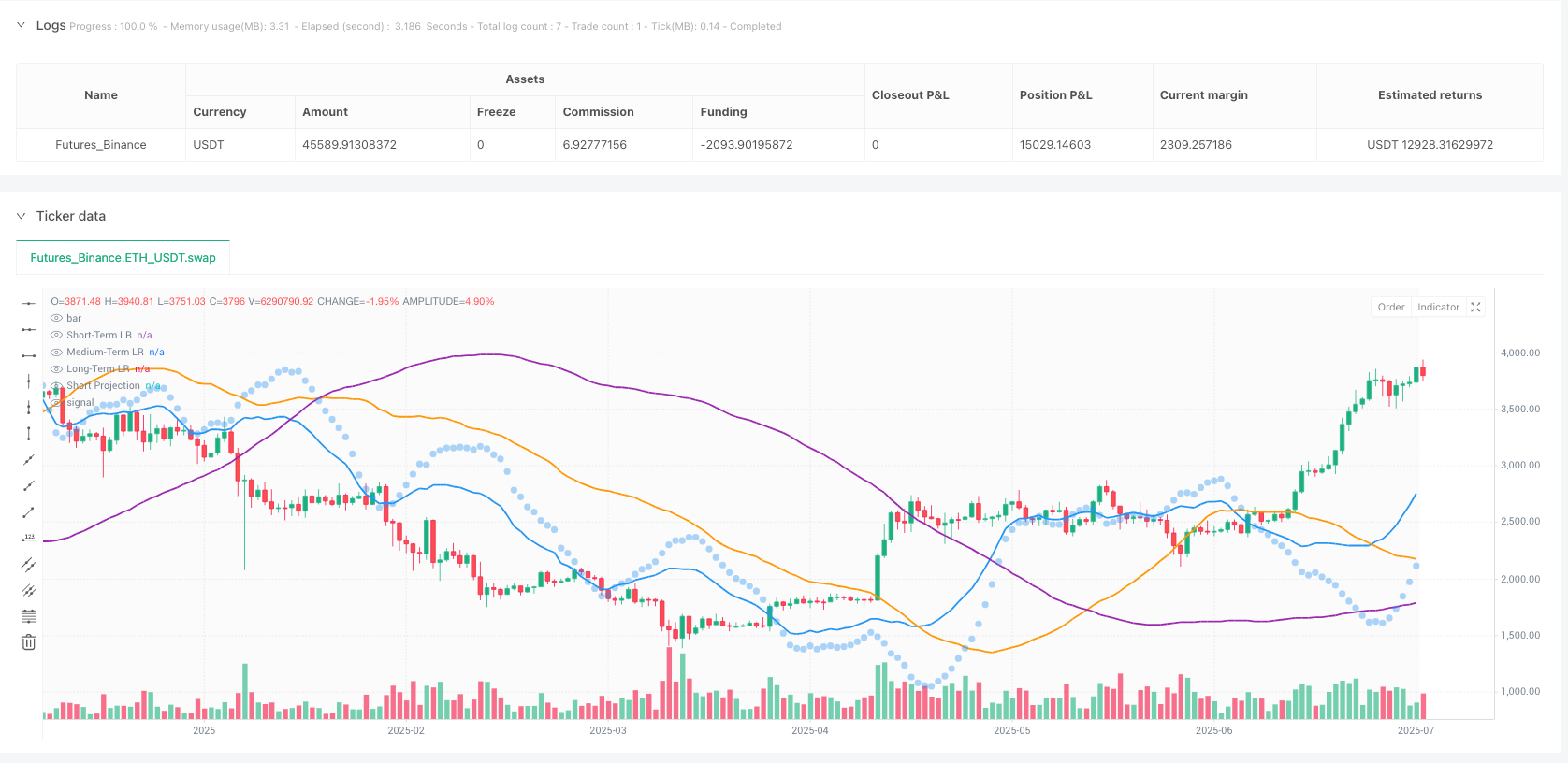
Visual Decision Support: The strategy provides real-time regression line plots (three layers in different colors), short-term projection markers, market bias background coloring, and a comprehensive statistics dashboard (R-squared metrics, validation scores, P&L status), offering intuitive support for trading decisions.
Strategy Risks
Despite its sophisticated design, the strategy faces the following potential risks:
Parameter Sensitivity: The strategy relies on multiple critical parameters (R-squared threshold, minimum correlation, slope threshold, etc.), which significantly impact performance. Inappropriate parameter settings may lead to overtrading or missed important signals. Solution: Optimize parameter settings through historical data backtesting and periodically reassess parameter effectiveness.
Market Condition Changes: The predictive capability of linear regression may significantly decrease during high volatility periods or sudden events, leading to poor strategy performance. Solution: Implement market state recognition mechanisms that automatically adjust or pause trading in non-linear market environments.
Statistical Lag: Linear regression analysis is inherently a lagging indicator, potentially responding too slowly in rapidly reversing markets. Solution: Consider integrating leading indicators or momentum indicators to increase sensitivity to market turning points.
Overfitting Risk: The multi-layer statistical framework may overfit to historical data, resulting in poor performance in future market environments. Solution: Implement forward testing and cross-validation to ensure strategy robustness and adaptability.
Computational Complexity: The strategy’s multi-layer regression analysis and statistical validation require significant computational resources, potentially facing execution delays in high-frequency trading environments. Solution: Optimize code efficiency and consider more efficient statistical computation methods.
Strategy Optimization Directions
Based on code analysis, the strategy can be optimized in the following directions:
Dynamic Timeframe Adaptation: Currently, the strategy uses fixed short/medium/long-term timeframe lengths. Consider automatically adjusting these parameters based on market volatility - shortening timeframes in high-volatility markets and extending them in low-volatility markets to better adapt to different market conditions.
Enhanced Prediction Models: The current strategy only uses linear regression. Consider integrating more complex models such as polynomial regression, ARIMA, or machine learning models (like random forests, support vector machines, etc.) to improve prediction accuracy.
Market Environment Classification: Add a market environment recognition module to distinguish between trending markets and range-bound markets, applying different trading logic and parameter settings in different market environments to enhance strategy adaptability.
Validation Mechanism Optimization: The current lookback validation is primarily based on short-term predictions. Extend this to all three timeframes and implement more sophisticated validation methods, such as rolling window cross-validation, to increase validation reliability.
Advanced Risk Management: Introduce more complex risk management techniques, such as dynamic stop-loss levels, volatility-adjusted position sizing, and risk parity across correlated assets, to further improve risk-adjusted returns.
Sentiment and Fundamental Integration: Consider integrating market sentiment indicators or fundamental factors into the model, such as volatility indices, interest rate differentials, or the impact of economic data releases, creating a more comprehensive trading decision framework.
Summary
The Multi-Layer Statistical Regression Trading Strategy is a technically advanced, meticulously designed quantitative trading system that provides a solid mathematical foundation for trading decisions through multi-layer linear regression analysis combined with rigorous statistical validation and intelligent risk control. The strategy’s greatest strength lies in its comprehensive market analysis capability and rigorous statistical methodology, effectively filtering out low-quality signals by simultaneously considering short-term, medium-term, and long-term price trends and subjecting them to statistical significance testing.
The strategy’s ensemble weighting mechanism and adaptive position management system enable it to dynamically adjust trading decisions and risk exposure based on signal quality, while the built-in lookback validation and daily loss limits provide additional safety measures. The comprehensive visualization interface and statistics dashboard also offer traders intuitive decision support tools.
Although the strategy faces potential risks related to parameter sensitivity, market condition adaptability, and statistical lag, its robustness and profitability can be further enhanced through regular parameter optimization, market environment classification, and prediction model enhancement. Overall, this is an advanced strategy that combines quantitative finance techniques with practical trading safeguards, particularly suitable for traders with some understanding of statistical methods.
/*backtest
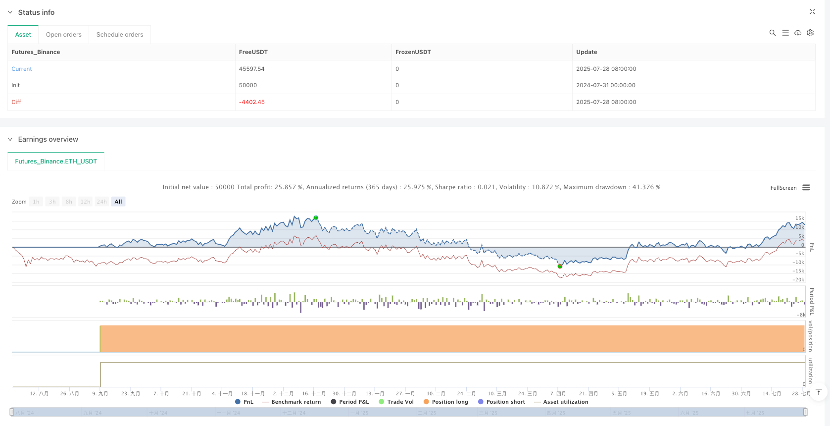
start: 2024-07-31 00:00:00
end: 2025-07-29 08:00:00
period: 1d
basePeriod: 1d
exchanges: [{"eid":"Futures_Binance","currency":"ETH_USDT"}]
*/
//@version=5
strategy("Multi-Layer Statistical Regression Strategy - Optimized", overlay=true)
// === MULTI-LAYER REGRESSION INPUTS ===
// Linear Regression Layers
lr_short_length = input.int(20, "Short-Term LR Length", minval=10, maxval=50, step=2)
lr_medium_length = input.int(50, "Medium-Term LR Length", minval=30, maxval=100, step=5)
lr_long_length = input.int(100, "Long-Term LR Length", minval=50, maxval=200, step=10)
// === 优化后的统计验证参数 (降低严格程度) ===
min_r_squared = input.float(0.45, "Min R-Squared Threshold", minval=0.2, maxval=0.8, step=0.05)
slope_threshold = input.float(0.00005, "Min Slope Significance", minval=0.00001, maxval=0.001, step=0.00001)
correlation_min = input.float(0.5, "Min Correlation", minval=0.3, maxval=0.8, step=0.05)
// Lookback/Look-Forward Analysis
validation_lookback = input.int(30, "Validation Lookback", minval=10, maxval=60, step=5)
prediction_horizon = input.int(10, "Prediction Horizon", minval=5, maxval=20, step=1)
// Ensemble Weights
weight_short = input.float(0.4, "Short-Term Weight", minval=0.1, maxval=0.6, step=0.1)
weight_medium = input.float(0.35, "Medium-Term Weight", minval=0.1, maxval=0.6, step=0.05)
weight_long = input.float(0.25, "Long-Term Weight", minval=0.1, maxval=0.6, step=0.05)
// === 优化后的风险管理参数 ===
position_size_pct = input.float(50.0, "Position Size %", minval=10.0, maxval=100.0, step=5.0)
max_daily_loss = input.float(12.0, "Max Daily Loss %", minval=5.0, maxval=25.0, step=2.5)
confidence_threshold = input.float(0.55, "Signal Confidence Threshold", minval=0.4, maxval=0.8, step=0.05)
// === 新增:信号强度分级 ===
use_graded_signals = input.bool(true, "Use Graded Signal Strength")
strong_signal_threshold = input.float(0.7, "Strong Signal Threshold", minval=0.6, maxval=0.9, step=0.05)
// === STATISTICAL FUNCTIONS ===
// Calculate Linear Regression with full statistics
linear_regression_stats(src, length) =>
var float sum_x = 0
var float sum_y = 0
var float sum_xy = 0
var float sum_x2 = 0
var float sum_y2 = 0
// Reset sums
sum_x := 0
sum_y := 0
sum_xy := 0
sum_x2 := 0
sum_y2 := 0
// Calculate sums for regression
for i = 0 to length - 1
x = i + 1
y = src[i]
if not na(y)
sum_x := sum_x + x
sum_y := sum_y + y
sum_xy := sum_xy + x * y
sum_x2 := sum_x2 + x * x
sum_y2 := sum_y2 + y * y
n = length
// Calculate regression coefficients
denominator = n * sum_x2 - sum_x * sum_x
slope = denominator != 0 ? (n * sum_xy - sum_x * sum_y) / denominator : 0
intercept = (sum_y - slope * sum_x) / n
// Calculate correlation coefficient (R)
correlation = (n * sum_xy - sum_x * sum_y) /
math.sqrt((n * sum_x2 - sum_x * sum_x) * (n * sum_y2 - sum_y * sum_y))
// Calculate R-squared
r_squared = correlation * correlation
// Current regression value
current_lr = intercept + slope * n
// Projected value (look-forward)
projected_lr = intercept + slope * (n + prediction_horizon)
[current_lr, slope, r_squared, correlation, projected_lr]
// === 优化后的统计显著性测试 (更灵活) ===
is_statistically_significant(r_squared, correlation, slope_abs, grade = "normal") =>
if grade == "relaxed"
r_squared >= (min_r_squared * 0.8) and math.abs(correlation) >= (correlation_min * 0.8) and math.abs(slope_abs) >= (slope_threshold * 0.5)
else if grade == "strict"
r_squared >= (min_r_squared * 1.2) and math.abs(correlation) >= (correlation_min * 1.1) and math.abs(slope_abs) >= (slope_threshold * 1.5)
else
r_squared >= min_r_squared and math.abs(correlation) >= correlation_min and math.abs(slope_abs) >= slope_threshold
// === MULTI-LAYER REGRESSION ANALYSIS ===
// Short-term layer
[lr_short, slope_short, r2_short, corr_short, proj_short] = linear_regression_stats(close, lr_short_length)
sig_short = is_statistically_significant(r2_short, corr_short, slope_short, "normal")
sig_short_strong = is_statistically_significant(r2_short, corr_short, slope_short, "strict")
// Medium-term layer
[lr_medium, slope_medium, r2_medium, corr_medium, proj_medium] = linear_regression_stats(close, lr_medium_length)
sig_medium = is_statistically_significant(r2_medium, corr_medium, slope_medium, "relaxed")
sig_medium_strong = is_statistically_significant(r2_medium, corr_medium, slope_medium, "normal")
// Long-term layer
[lr_long, slope_long, r2_long, corr_long, proj_long] = linear_regression_stats(close, lr_long_length)
sig_long = is_statistically_significant(r2_long, corr_long, slope_long, "relaxed")
// === LOOKBACK VALIDATION ===
validate_prediction_accuracy() =>
var array<float> accuracy_scores = array.new<float>()
if bar_index >= validation_lookback
historical_slope = (close - close[prediction_horizon]) / prediction_horizon
predicted_slope = slope_short[prediction_horizon]
error = math.abs(historical_slope - predicted_slope)
accuracy = math.max(0, 1 - error * 10000)
array.push(accuracy_scores, accuracy)
if array.size(accuracy_scores) > validation_lookback
array.shift(accuracy_scores)
array.size(accuracy_scores) > 5 ? array.avg(accuracy_scores) : 0.5
validation_accuracy = validate_prediction_accuracy()
// === 优化后的集成信号生成 ===
// Individual layer signals (directional)
signal_short = sig_short ? (slope_short > 0 ? 1 : -1) : 0
signal_medium = sig_medium ? (slope_medium > 0 ? 1 : -1) : 0
signal_long = sig_long ? (slope_long > 0 ? 1 : -1) : 0
// Weighted ensemble score
ensemble_score = (signal_short * weight_short +
signal_medium * weight_medium +
signal_long * weight_long)
// === 多级信号置信度计算 ===
// 基础一致性评分
agreement_score = math.abs(signal_short + signal_medium + signal_long) / 3.0
// 统计置信度 (使用加权平均)
stat_confidence = (r2_short * weight_short +
r2_medium * weight_medium +
r2_long * weight_long)
// 验证置信度
validation_confidence = validation_accuracy
// 整体置信度 (调整权重比例)
overall_confidence = (agreement_score * 0.3 +
stat_confidence * 0.5 +
validation_confidence * 0.2)
// 信号强度分级
signal_strength = math.abs(ensemble_score)
is_strong_signal = overall_confidence > strong_signal_threshold and (sig_short_strong or sig_medium_strong)
// === POSITION MANAGEMENT ===
trend_direction = ensemble_score > 0 ? 1 : ensemble_score < 0 ? -1 : 0
// 基于信号强度的仓位调整
confidence_multiplier = if use_graded_signals
if is_strong_signal
1.0 + (overall_confidence - strong_signal_threshold) * 0.5
else
0.7 + (overall_confidence / strong_signal_threshold) * 0.3
else
overall_confidence > confidence_threshold ? 1.0 : overall_confidence / confidence_threshold
base_position_value = strategy.equity * (position_size_pct / 100)
adjusted_position_value = base_position_value * confidence_multiplier
position_units = adjusted_position_value / close
// Daily loss tracking
var float daily_start_equity = strategy.equity
if ta.change(time("1D"))
daily_start_equity := strategy.equity
current_daily_loss = daily_start_equity > 0 ? (daily_start_equity - strategy.equity) / daily_start_equity * 100 : 0
halt_trading = current_daily_loss > max_daily_loss
// === 优化后的入场/退出逻辑 ===
// 更灵活的入场条件
long_condition_basic = ensemble_score > 0.2 and overall_confidence > confidence_threshold and sig_short
long_condition_strong = ensemble_score > 0.4 and overall_confidence > strong_signal_threshold and sig_short and sig_medium
short_condition_basic = ensemble_score < -0.2 and overall_confidence > confidence_threshold and sig_short
short_condition_strong = ensemble_score < -0.4 and overall_confidence > strong_signal_threshold and sig_short and sig_medium
// 入场信号生成
long_signal = use_graded_signals ? (long_condition_strong or long_condition_basic) : long_condition_strong
short_signal = use_graded_signals ? (short_condition_strong or short_condition_basic) : short_condition_strong
// 策略执行
if long_signal and not halt_trading and strategy.position_size <= 0
signal_type = long_condition_strong ? "Strong Long" : "Basic Long"
strategy.entry("Long", strategy.long, qty=position_units,
comment=signal_type + ": " + str.tostring(overall_confidence, "#.##"))
if short_signal and not halt_trading and strategy.position_size >= 0
signal_type = short_condition_strong ? "Strong Short" : "Basic Short"
strategy.entry("Short", strategy.short, qty=position_units,
comment=signal_type + ": " + str.tostring(overall_confidence, "#.##"))
// 降低初始化门槛
if strategy.position_size == 0 and not halt_trading and barstate.isconfirmed
if ensemble_score > 0.15 and overall_confidence > (confidence_threshold * 0.8)
strategy.entry("InitLong", strategy.long, qty=position_units * 0.8, comment="Init Long")
else if ensemble_score < -0.15 and overall_confidence > (confidence_threshold * 0.8)
strategy.entry("InitShort", strategy.short, qty=position_units * 0.8, comment="Init Short")
// Emergency exit
if halt_trading and strategy.position_size != 0
strategy.close_all(comment="Daily Loss Limit")
// === 增强的可视化 ===
// Plot regression lines with transparency based on significance
plot(lr_short, "Short-Term LR", color=sig_short_strong ? color.blue : color.new(color.blue, 50), linewidth=2)
plot(lr_medium, "Medium-Term LR", color=sig_medium_strong ? color.orange : color.new(color.orange, 50), linewidth=2)
plot(lr_long, "Long-Term LR", color=color.new(color.purple, 30), linewidth=1)
// Background with graded confidence
bg_color = if overall_confidence > strong_signal_threshold
ensemble_score > 0 ? color.new(color.green, 85) : color.new(color.red, 85)
else if overall_confidence > confidence_threshold
ensemble_score > 0 ? color.new(color.green, 92) : color.new(color.red, 92)
else
color.new(color.gray, 97)
bgcolor(bg_color)
// Enhanced signal markers
plotshape(long_condition_strong, "Strong Long", shape.triangleup, location.belowbar,
color=color.green, size=size.large)
plotshape(long_condition_basic and not long_condition_strong, "Basic Long", shape.triangleup, location.belowbar,
color=color.new(color.green, 40), size=size.small)
plotshape(short_condition_strong, "Strong Short", shape.triangledown, location.abovebar,
color=color.red, size=size.large)
plotshape(short_condition_basic and not short_condition_strong, "Basic Short", shape.triangledown, location.abovebar,
color=color.new(color.red, 40), size=size.small)