
Strategy Overview
The Multi-Dimensional Game Theory Trading Strategy is a quantitative trading approach that combines game theory principles with technical analysis, primarily identifying high-probability trading opportunities by analyzing crowd behavior, institutional fund flows, liquidity traps, and Nash equilibrium states. This strategy is built on the core concept that financial markets represent a game between different participants, and by analyzing the behavioral patterns and decision tendencies of these participants, potential market movements can be predicted. The strategy employs automated trading logic combined with a dynamic risk management system, aiming to capture market inefficiencies caused by retail panic, institutional fund movements, and liquidity traps.
Strategy Principles
The strategy employs a multi-layered game theory analytical framework, analyzing the market through four key dimensions:
-
Crowd Behavior Detection: The strategy uses the RSI indicator (default 14 periods) combined with volume analysis to identify herd panic or greed in the market. When RSI exceeds 70 and volume is significantly higher than its 20-period moving average (default 2x), the system identifies retail crowd buying; when RSI falls below 30 with similar volume anomalies, it identifies retail panic selling. These extreme conditions often indicate potential market reversals.
-
Liquidity Trap Analysis: The strategy scans recent highs and lows (default 50 periods) to identify potential "stop-loss hunting" zones. When price breaks above a recent high but subsequently closes below it, accompanied by increased volume, the system recognizes a potential upward liquidity trap; the reverse applies for downward traps. These traps are typically set by large institutions to trigger retail stop-loss orders.
-
Institutional Fund Flow Analysis: By monitoring abnormally large volume (default 2.5x the average) and the Accumulation/Distribution indicator (A/D line), the strategy tracks institutional activity. An A/D line above its 21-period moving average with large volume is identified as institutional accumulation; the opposite indicates distribution. Additionally, the strategy uses a Smart Money Index ((close-open)/(high-low)*volume) to confirm smart money direction.
-
Nash Equilibrium Calculation: Based on the 100-period moving average and standard deviation of price, the strategy calculates a statistically significant "equilibrium band." When price is within this band, the market is viewed as stable; when price significantly deviates from the band, it's considered overbought or oversold, with potential for regression to equilibrium.
Based on the analysis of these four dimensions, the strategy generates three types of trading signals:
- Contrarian Signals: When retail exhibits herd selling, accompanied by institutional accumulation or a downward liquidity trap, a buy signal is generated; the reverse produces a sell signal.
- Momentum Signals: When price is below the Nash equilibrium band, with a positive Smart Money Index and no retail herd buying, a buy signal is generated; the reverse produces a sell signal.
- Equilibrium Reversion Signals: When price is below the Nash equilibrium band and shows an upward trend (closing price higher than previous period) with volume above average, a buy signal is generated; the reverse produces a sell signal.
The final multi-dimensional game theory trading decision is derived from these three types of signals and adjusted through a dynamic position management system based on the minimax principle.
Strategy Advantages
-
Comprehensive Multi-dimensional Market Information: The strategy not only focuses on basic technical indicators like price and volume but also incorporates market participant behavior patterns, institutional fund flows, liquidity traps, and statistical equilibrium, providing a more comprehensive understanding of the market.
-
Adaptation to Different Market Conditions: Through the game theory framework, the strategy can adaptively adjust to different market environments. In Nash equilibrium zones, the strategy takes a conservative stance; when institutional activity is detected, the strategy becomes more aggressive; during retail panic, the strategy takes contrarian positions.
-
Dynamic Risk Management: The strategy includes a comprehensive risk control mechanism, featuring automatic stop-loss (default 2%), take-profit targets (default 5%), and dynamic position adjustment based on market conditions, adhering to the minimax principle to protect capital while optimizing returns.
-
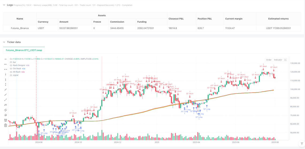
Visualization Decision Support: The strategy provides rich visualization elements, including Nash equilibrium bands, background color indicators (red for crowd buying, green for crowd selling, blue for institutional activity), and signal markers. Additionally, two information panels intuitively display game theory status and backtest performance data.
-
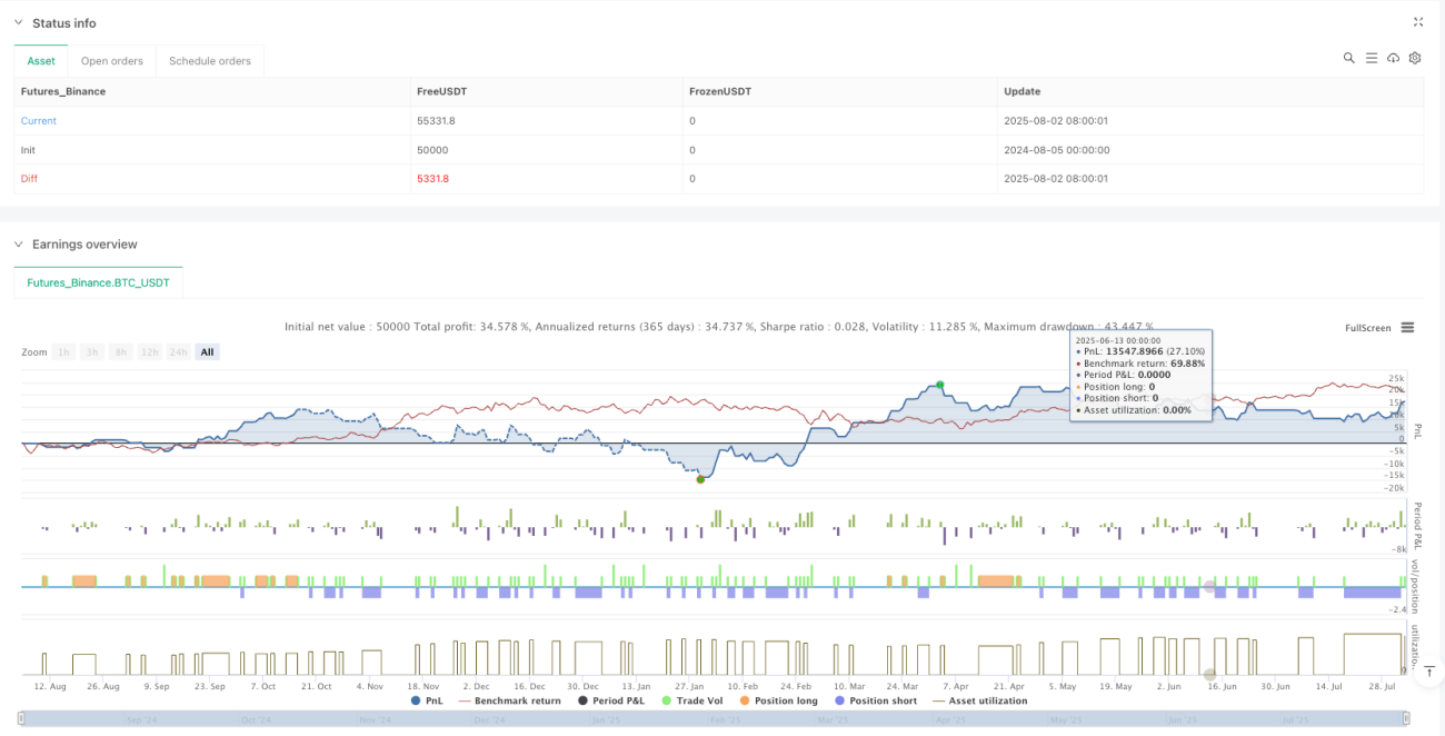
Complete Backtesting Framework: The strategy incorporates a comprehensive backtesting analysis system, tracking key metrics such as total trades, win rate, net profit, profit factor, and maximum drawdown, facilitating strategy optimization and performance evaluation.
Strategy Risks
-
Parameter Sensitivity: The effectiveness of the strategy heavily depends on precise parameter settings. RSI periods, volume multiplier thresholds, liquidity lookback periods, Nash equilibrium deviations, and other parameters need adjustment according to different markets and timeframes. Inappropriate parameter settings may lead to excessive false signals or missed trading opportunities.
-
Market Noise Interference: In short timeframes (such as minute-level), market noise can cause misidentification of crowd behavior and liquidity traps. The strategy is best applied to medium to long-term timeframes such as H1 (1 hour) to D1 (daily) to filter out short-term fluctuation interference.
-
Overtrading Risk: Since the strategy combines three signal sources, it may generate excessive trading signals under certain market conditions, leading to overtrading and commission erosion. It's recommended to add signal filtering mechanisms, such as signal confirmation periods or strength thresholds.
-
Systemic Risk Exposure: The strategy primarily relies on technical indicators and behavioral analysis, lacking adaptability to systemic risk factors such as macroeconomic events, policy changes, or major news. During significant market events, the strategy may fail to correctly assess risks and potentially suffer substantial losses.
-
Backtesting vs. Real Trading Differences: Backtest results may suffer from look-ahead bias or overfitting to historical data. Real trading may face slippage, insufficient liquidity, or execution delays not reflected in backtesting.
Optimization Directions
-
Machine Learning Enhancement: Introduce machine learning algorithms to optimize parameter selection and signal generation processes. Through supervised learning or reinforcement learning methods, parameters can be automatically adjusted according to different market environments, improving strategy adaptability and robustness.
-
Multi-timeframe Analysis Integration: Add multi-timeframe analysis to the strategy, for example, simultaneously considering signals from daily, 4-hour, and 1-hour levels, executing trades only when signals from multiple timeframes align, reducing false signals and increasing trade success rates.
-
Volatility Adjustment Mechanism: Dynamically adjust stop-loss levels, take-profit percentages, and position sizes based on market volatility. Tighten risk controls in high-volatility environments and moderately relax parameters in low-volatility environments to adapt to different market conditions.
-
Fundamental Data Integration: Incorporate macroeconomic indicators, market sentiment indices, or news sentiment analysis into the decision framework, creating a more comprehensive trading system that considers both technical and behavioral factors as well as fundamental factors.
-
Adaptive Filters: Develop adaptive signal filtering systems that dynamically adjust signal thresholds based on historical signal performance, filtering out low-probability trading opportunities and concentrating resources on high-probability trades, thereby improving overall profitability and capital efficiency.
-
Nash Equilibrium Improvement: Optimize the Nash equilibrium calculation method, considering the introduction of non-linear statistical models or adaptive equilibrium bandwidth, making equilibrium judgments more accurate, especially during market transitions or high-volatility periods.
Conclusion
The Multi-Dimensional Game Theory Trading Strategy provides traders with a unique market analysis framework by combining classical game theory principles with modern quantitative analysis techniques. By simultaneously monitoring retail behavior, institutional activity, liquidity traps, and statistical equilibrium states, the strategy attempts to find order in chaotic markets and gain advantages from the games between market participants.
The core advantages of the strategy lie in its multi-dimensional analysis capabilities and dynamic risk management system, enabling it to adapt to different market environments and provide relatively robust risk-adjusted returns. However, the complexity of the strategy also brings challenges in parameter optimization and potential overfitting risks.
For traders wishing to apply this strategy, it is recommended to first conduct thorough backtesting across different markets and timeframes, adjust parameters to suit the characteristics of specific trading instruments, and consider implementing the optimization directions proposed in this article. Additionally, using this strategy as part of a broader trading system, rather than as a sole decision basis, may yield better results.
Through continuous improvement and optimization, the Multi-Dimensional Game Theory Trading Strategy has the potential to become a powerful weapon in a trader's toolkit, helping to gain sustained competitive advantages in complex and dynamic financial markets.
/*backtest
start: 2024-08-21 02:40:00
end: 2025-08-03 08:00:00
period: 1d
basePeriod: 1h
exchanges: [{"eid":"Futures_Binance","currency":"BTC_USDT"}]
args: [["v_input_int_2",5],["v_input_int_3",5]]
*/

//@version=5
strategy("Game Theory Trading Strategy", overlay=true, initial_capital=10000, pyramiding=3, default_qty_type=strategy.percent_of_equity, default_qty_value=10)
- 1