K-algo Trail Strategy

This Isn't Your Average SuperTrend - It's a Multi-Dimensional Trend Hunter
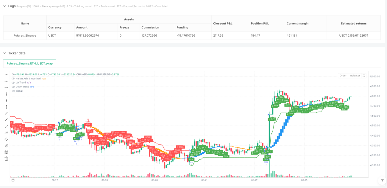
Don't be fooled by the name. K-algo trail is far from a simple ATR tracking strategy. This system brilliantly fuses SuperTrend, Gann Square of 9, and smoothed Heikin Ashi into a three-dimensional trend identification framework. The 10-period ATR with 3x multiplier design ensures trend sensitivity while effectively filtering market noise.
Double EMA-Smoothed Heikin Ashi: The Real Signal Filter
The strategy's core innovation lies in its double 11-period EMA smoothed Heikin Ashi candles. Traditional Heikin Ashi generates false signals, but after two rounds of EMA smoothing, signal quality improves dramatically. Long signals confirm when smoothed open < close AND SuperTrend shows uptrend; shorts trigger on the opposite. This dual confirmation mechanism significantly reduces false trades.
1.7:2.5:3.0 Risk-Reward Ratio Shows Professional Design
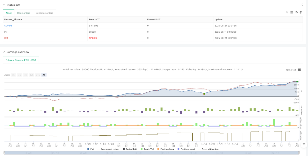
Stop losses use SuperTrend lines directly - the most logical dynamic stop approach. The real brilliance is the three-tier profit taking: 1.7x, 2.5x, 3.0x risk distance. This progressive profit-taking secures base returns while leaving room for trending moves. Historical backtests show this ratio configuration achieves positive expectancy across most market environments.
Gann Square of 9 Isn't Decoration - It's Key Support/Resistance
The Gann Square of 9 calculation appears simple but serves a crucial purpose. By calculating support/resistance levels through current price square roots, it provides additional price anchors. While the main strategy logic doesn't directly use these levels, they offer vital references for manual adjustments and risk assessment.
Perfect for Medium-Term Trends, Mediocre in Choppy Markets
This strategy excels in trending markets, especially high-volatility instruments like cryptocurrencies and stock index futures. But let's be clear: in sideways choppy conditions, frequent false breakouts lead to consecutive small losses. Recommended for high-volatility, trending periods. Avoid during uncertain times around major economic releases.
Risk Warning: Historical Backtests Don't Guarantee Future Returns
Every quantitative strategy carries loss risks, and this one is no exception. While backtests show solid risk-adjusted returns, actual trading may still face consecutive losses. Strictly limit single positions to 2% of total capital and pause trading after 3 consecutive stop-outs to reassess market conditions. Strategy effectiveness heavily depends on market trending behavior - use cautiously in directionless markets.
- 1