
In quantitative trading, we often face a core problem: single technical indicators are prone to generating false signals in market noise, leading to frequent stop-losses and capital drawdowns. So, how can we build a trading system that captures trends while effectively filtering noise?
The Gaussian Channel multi-filter strategy analyzed today provides a solution worth deep study by cleverly combining four different dimensions of technical indicators.
1. Gaussian Channel - Trend Identification Core
The strategy’s foundation is a 4-pole Gaussian filter with a 144-period sampling window. Unlike traditional moving averages, the Gaussian filter eliminates most market noise through mathematical modeling while maintaining sensitivity to price changes.
Key parameter settings: - Gaussian poles: 4 (balancing lag and smoothness) - Sampling period: 144 (capturing medium-term trends) - Filter multiplier: 1.414 (standard deviation multiple, controlling channel width)
2. Kijun-Sen Line (130-period) - Medium-to-Long-term Trend Confirmation
This uses a 130-period Kijun-Sen line as a trend filter, rather than the traditional 26-period. What’s the significance of this adjustment?
Longer period settings can: - Reduce false breakout signals - Ensure trading direction aligns with the main trend - Improve signal quality and reduce trading frequency
3. VAPI Indicator - Volume Price Analysis
VAPI (Volume Adjusted Price Indicator) analyzes the relationship between volume and price changes to determine market participants’ true intentions. When VAPI > 0, it supports long positions; when < 0, it supports short positions.
4. ATR Dynamic Stop Loss - Risk Control Mechanism
Using 4.5 times the 11-period ATR as stop-loss distance, this setting considers market volatility while avoiding overly tight stops being triggered by market noise.
The most valuable aspect of this strategy lies in its unique capital management approach:
Position Splitting Logic: - 75% position: Fixed 3.5x risk-reward ratio take profit - 25% position: Dynamic trailing stop loss
Why This Design?
1. Entry Risk Control - Each trade risk limited to 3% of account capital - Dynamic position sizing based on ATR
2. Position Risk Management - Main stop loss: 4.5x ATR - Trailing stop: Dynamic adjustment, locking in floating profits - Additional take profit: 10% fixed profit protection
3. Signal Filtering Mechanism Four technical indicators confirm simultaneously, significantly reducing false signal probability.
Core Advantages:
Potential Limitations:
1. Instrument Selection Prioritize instruments with strong trending characteristics, such as major currency pairs, stock index futures, etc.
2. Parameter Optimization Recommend backtesting optimization based on historical data of specific trading instruments, particularly focusing on: - Gaussian channel sampling period - Kijun-Sen period length - ATR stop loss multiplier
3. Market Environment Adaptation In obvious ranging markets, consider pausing the strategy or adjusting parameter settings.
The value of this strategy lies not only in its technical implementation but also in the systematic thinking it embodies:
For quantitative traders, this strategy provides an excellent framework reference. The key is not copying parameters but understanding the design philosophy and making appropriate adjustments based on your trading instruments and risk preferences.
Remember, the best strategy is not the most complex one, but the one most suitable for your trading style and market environment.
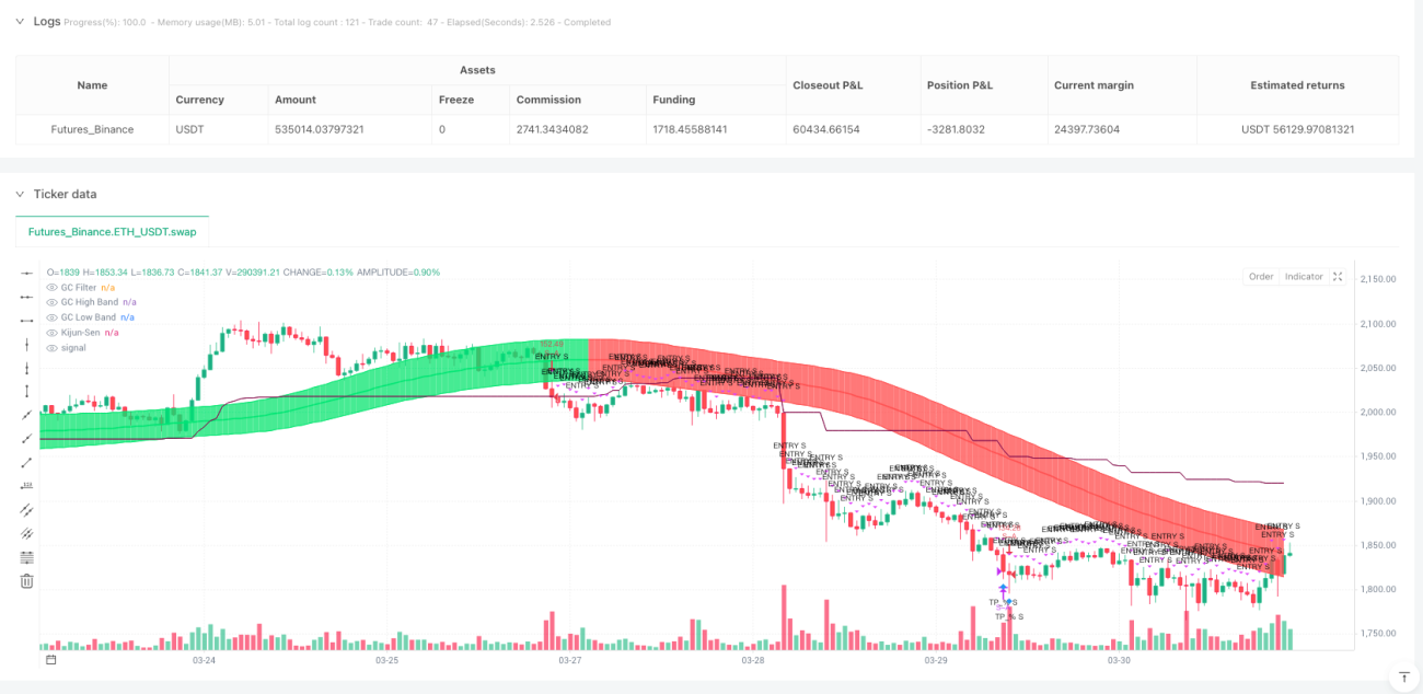
/*backtest
start: 2025-01-01 00:00:00
end: 2025-04-01 00:00:00
period: 1h
basePeriod: 1h
exchanges: [{"eid":"Futures_Binance","currency":"ETH_USDT","balance":500000}]
*/
// @version=6
strategy("Gaussian Channel Strategy – GC + Kijun (120) + VAPI Gate + ATR(4.5x) + 75/25 TP-TRAIL + Extra %TP",
overlay=true)
// =============================
// ======= INPUTS ==============
// =============================
N_poles = input.int(4, "Gaussian Poles", minval=1, maxval=9)
per = input.int(144, "Sampling Period", minval=2)
mult = input.float(1.414, "Filtered TR Multiplier", step=0.001)
src = input.source(hlc3, "Source")
modeLag = input.bool(false, "Reduced Lag Mode")
modeFast = input.bool(false, "Fast Response Mode")
kijunLen = input.int(130, "Kijun-Sen Period")
vapiLen = input.int(10, "VAPI Length")
vapiThresh= input.float(0.0, "VAPI Threshold (0 = zero line)")
atrLen = input.int(11, "ATR Length (RMA)")
slATRmul = input.float(4.5, "SL = ATR ×", step=0.1)
rr_fixed = input.float(3.5, "Fixed TP RR (Leg A)", step=0.1)
allocA = input.float(75, "Allocation %: Fixed TP Leg", minval=1, maxval=99)
riskPct = input.float(3.0, "Risk % of Equity per Trade", step=0.1, minval=0.1, maxval=10)
tpEnable = input.bool(true, "Enable Extra % Take Profit")
tpPctLong = input.float(10.0, "Extra Long TP % of Entry", step=0.1, minval=0)
tpPctShort = input.float(10.0, "Extra Short TP % of Entry", step=0.1, minval=0)
// =============================
// ===== CORE COMPONENTS =======
// =============================
atr = ta.rma(ta.tr(true), atrLen)
donchian_avg(len) => (ta.highest(high, len) + ta.lowest(low, len)) / 2.0
kijun = donchian_avg(kijunLen)
// --- VAPI_LB (LazyBear) ---
rs(x, len) => ta.cum(x) - nz(ta.cum(x)[len])
v_x = (2*close - high - low) / math.max(high - low, syminfo.mintick)
v_tva = rs(volume * v_x, vapiLen)
v_tv = rs(volume, vapiLen)
v_va = 100 * (v_tva / v_tv)
// =============================
// ===== Gaussian Channel ======
// =============================
f_filt9x(_a, _s, _i) =>
int _m2 = 0, int _m3 = 0, int _m4 = 0, int _m5 = 0, int _m6 = 0,
int _m7 = 0, int _m8 = 0, int _m9 = 0, float _f = 0.0, _x = (1 - _a)
_m2 := _i == 9 ? 36 : _i == 8 ? 28 : _i == 7 ? 21 : _i == 6 ? 15 : _i == 5 ? 10 : _i == 4 ? 6 : _i == 3 ? 3 : _i == 2 ? 1 : 0
_m3 := _i == 9 ? 84 : _i == 8 ? 56 : _i == 7 ? 35 : _i == 6 ? 20 : _i == 5 ? 10 : _i == 4 ? 4 : _i == 3 ? 1 : 0
_m4 := _i == 9 ? 126 : _i == 8 ? 70 : _i == 7 ? 35 : _i == 6 ? 15 : _i == 5 ? 5 : _i == 4 ? 1 : 0
_m5 := _i == 9 ? 126 : _i == 8 ? 56 : _i == 7 ? 21 : _i == 6 ? 6 : _i == 5 ? 1 : 0
_m6 := _i == 9 ? 84 : _i == 8 ? 28 : _i == 7 ? 7 : _i == 6 ? 1 : 0
_m7 := _i == 9 ? 36 : _i == 8 ? 8 : _i == 7 ? 1 : 0
_m8 := _i == 9 ? 9 : _i == 8 ? 1 : 0
_m9 := _i == 9 ? 1 : 0
_f := math.pow(_a, _i) * nz(_s) +
_i * _x * nz(_f[1]) - (_i >= 2 ?
_m2 * math.pow(_x, 2) * nz(_f[2]) : 0) + (_i >= 3 ?
_m3 * math.pow(_x, 3) * nz(_f[3]) : 0) - (_i >= 4 ?
_m4 * math.pow(_x, 4) * nz(_f[4]) : 0) + (_i >= 5 ?
_m5 * math.pow(_x, 5) * nz(_f[5]) : 0) - (_i >= 6 ?
_m6 * math.pow(_x, 6) * nz(_f[6]) : 0) + (_i >= 7 ?
_m7 * math.pow(_x, 7) * nz(_f[7]) : 0) - (_i >= 8 ?
_m8 * math.pow(_x, 8) * nz(_f[8]) : 0) + (_i == 9 ?
_m9 * math.pow(_x, 9) * nz(_f[9]) : 0)
f_pole(_a, _s, _i) =>
_f1 = f_filt9x(_a, _s, 1), _f2 = (_i >= 2 ? f_filt9x(_a, _s, 2) : 0), _f3 = (_i >= 3 ? f_filt9x(_a, _s, 3) : 0)
_f4 = (_i >= 4 ? f_filt9x(_a, _s, 4) : 0), _f5 = (_i >= 5 ? f_filt9x(_a, _s, 5) : 0), _f6 = (_i >= 6 ? f_filt9x(_a, _s, 6) : 0)
_f7 = (_i >= 7 ? f_filt9x(_a, _s, 7) : 0), _f8 = (_i >= 8 ? f_filt9x(_a, _s, 8) : 0), _f9 = (_i == 9 ? f_filt9x(_a, _s, 9) : 0)
_fn = _i == 1 ? _f1 : _i == 2 ? _f2 : _i == 3 ? _f3 : _i == 4 ? _f4 : _i == 5 ? _f5 : _i == 6 ? _f6 : _i == 7 ? _f7 : _i == 8 ? _f8 : _i == 9 ? _f9 : na
[_fn, _f1]
beta = (1 - math.cos(4*math.asin(1)/per)) / (math.pow(1.414, 2/N_poles) - 1)
alpha = - beta + math.sqrt(math.pow(beta, 2) + 2*beta)
lag = (per - 1) / (2.0 * N_poles)
srcdata = modeLag ? src + (src - nz(src[lag])) : src
tr_raw = ta.tr(true)
trdata = modeLag ? tr_raw + (tr_raw - nz(tr_raw[lag])) : tr_raw
[filt_n, filt_1] = f_pole(alpha, srcdata, N_poles)
[filt_n_tr, filt_1_tr] = f_pole(alpha, trdata, N_poles)
filt = modeFast ? (filt_n + filt_1)/2.0 : filt_n
filttr = modeFast ? (filt_n_tr + filt_1_tr)/2.0 : filt_n_tr
hband = filt + filttr * mult
lband = filt - filttr * mult
// =============================
// ===== Signals & Filters =====
// =============================
doLong = close > filt and close > kijun and v_va > vapiThresh
doShort = close < filt and close < kijun and v_va < -vapiThresh
// =============================
// ===== Position Sizing =======
// =============================
riskValue = strategy.equity * (riskPct/100.0)
slDist = atr * slATRmul
qtyTotal = slDist > 0 ? riskValue / slDist : 0.0
qtyA = qtyTotal * (allocA/100.0)
qtyB = qtyTotal * ((100 - allocA)/100.0)
// =============================
// ===== Order Execution =======
// =============================
var float trailStopL = na
var float trailStopS = na
inLong = strategy.position_size > 0
inShort = strategy.position_size < 0
entryPx = strategy.position_avg_price
// Entries
if doLong and not inLong and strategy.position_size <= 0
strategy.order("L-A", strategy.long, qty=qtyA)
strategy.order("L-B", strategy.long, qty=qtyB)
trailStopL := na
if doShort and not inShort and strategy.position_size >= 0
strategy.order("S-A", strategy.short, qty=qtyA)
strategy.order("S-B", strategy.short, qty=qtyB)
trailStopS := na
// LONG management
if inLong
slL = entryPx - slDist
tpA = entryPx + rr_fixed * slDist
// Leg A: 固定RR止盈 + 止损
strategy.exit("TP/SL-LA", from_entry="L-A", limit=tpA, stop=slL)
// Leg B: 追踪止损
trailStopL := na(trailStopL[1]) or strategy.position_size[1] <= 0 ? slL : math.max(trailStopL[1], close - slDist)
strategy.exit("Trail-LB", from_entry="L-B", stop=trailStopL)
// 额外百分比止盈
if tpEnable and high >= entryPx * (1 + tpPctLong/100.0)
strategy.close("L-A", comment="ExtraTP")
strategy.close("L-B", comment="ExtraTP")
// SHORT management
if inShort
slS = entryPx + slDist
tpA = entryPx - rr_fixed * slDist
// Leg A: 固定RR止盈 + 止损
strategy.exit("TP/SL-SA", from_entry="S-A", limit=tpA, stop=slS)
// Leg B: 追踪止损
trailStopS := na(trailStopS[1]) or strategy.position_size[1] >= 0 ? slS : math.min(trailStopS[1], close + slDist)
strategy.exit("Trail-SB", from_entry="S-B", stop=trailStopS)
// 额外百分比止盈
if tpEnable and low <= entryPx * (1 - tpPctShort/100.0)
strategy.close("S-A", comment="ExtraTP")
strategy.close("S-B", comment="ExtraTP")
// =============================
// ===== 图表绘制 ==============
// =============================
fcolor = filt > nz(filt[1]) ? color.new(color.lime, 0) : filt < nz(filt[1]) ? color.new(color.red, 0) : color.new(color.gray, 0)
plotFilter = plot(filt, title="GC Filter", color=fcolor, linewidth=2)
plotH = plot(hband, title="GC High Band", color=fcolor)
plotL = plot(lband, title="GC Low Band", color=fcolor)
fill(plotH, plotL, color=color.new(fcolor, 80))
plot(kijun, "Kijun-Sen", color=color.new(color.maroon, 0))
// 信号标记
plotshape(doLong, title="Long Setup", style=shape.triangleup, location=location.belowbar, color=color.new(color.lime, 0), size=size.tiny, text="ENTRY L")
plotshape(doShort, title="Short Setup", style=shape.triangledown, location=location.abovebar, color=color.new(color.fuchsia, 0), size=size.tiny, text="ENTRY S")