AR-GARCH Time Series Forecasting Strategy


Created on: 2025-09-09 16:39:24 Modified on: 2025-09-12 13:27:12
Copy: 0 Number of hits: 58
avatar of ianzeng123 ianzeng123
2
Follow
319
Followers

 AR-GARCH Time Series Forecasting Strategy  AR-GARCH Time Series Forecasting Strategy

Why Do Traditional Technical Analysis Methods Fail in Complex Markets?

In quantitative trading, we often encounter this puzzle: why do strategies based on simple moving averages or RSI perform excellently in certain market environments, yet frequently fail in others? The answer lies in the complexity of financial time series—they not only exhibit autocorrelation but also feature time-varying volatility characteristics.

The strategy we’re analyzing today cleverly combines an AR(2) autoregressive model with a GARCH(1,1) conditional heteroskedasticity model, attempting to solve this problem from a statistical perspective. This isn’t a simple overlay of technical indicators, but rather a deep exploration of the essential characteristics of financial time series.

How Does the AR(2) Model Capture Price Memory Effects?

The strategy’s core lies in the application of the AR(2) autoregressive model. What is autoregression? Simply put, it’s using the past self to predict the future self. The AR(2) model assumes that current returns can be linearly represented by the previous two periods’ returns:

r_t = φ₁ × r_{t-1} + φ₂ × r_{t-2} + ε_t

The code solves for coefficients φ₁ and φ₂ through Yule-Walker equations:

c0 = calcAutoCovariance(returns, 0, lengthReg) // Lag-0 autocovariance
c1 = calcAutoCovariance(returns, 1, lengthReg) // Lag-1 autocovariance  
c2 = calcAutoCovariance(returns, 2, lengthReg) // Lag-2 autocovariance
phi1 = (c1 * c0 - c2 * c1) / denominator // First autoregressive coefficient
phi2 = (c2 * c0 - c1 * c1) / denominator // Second autoregressive coefficient

The advantage of this approach is that it doesn’t rely on subjective judgment, but lets the data “speak” for itself, discovering the inherent patterns in price series.

Why Can GARCH Models Better Characterize Market Risk?

AR models alone are insufficient because financial market volatility is not constant. We all know the “volatility clustering” phenomenon—large fluctuations often follow large fluctuations, while calm periods tend to persist for longer durations.

The GARCH(1,1) model is designed precisely to characterize this feature:

σ²_t = ω + α × ε²_{t-1} + β × σ²_{t-1}

The implementation logic in the code clearly reflects this:

omega = (1 - adjustedAlpha - adjustedBeta) * longTermVar
garchVariance := omega + adjustedAlpha * math.pow(arResidual[1], 2) + adjustedBeta * garchVariance[1]

The key insight here is that current conditional variance depends not only on the previous period’s squared residual (short-term shock) but also on the previous period’s conditional variance (long-term persistence). Parameter α controls the impact of short-term shocks, while β controls volatility persistence.

How Does the Strategy’s Trading Logic Achieve Risk-Return Balance?

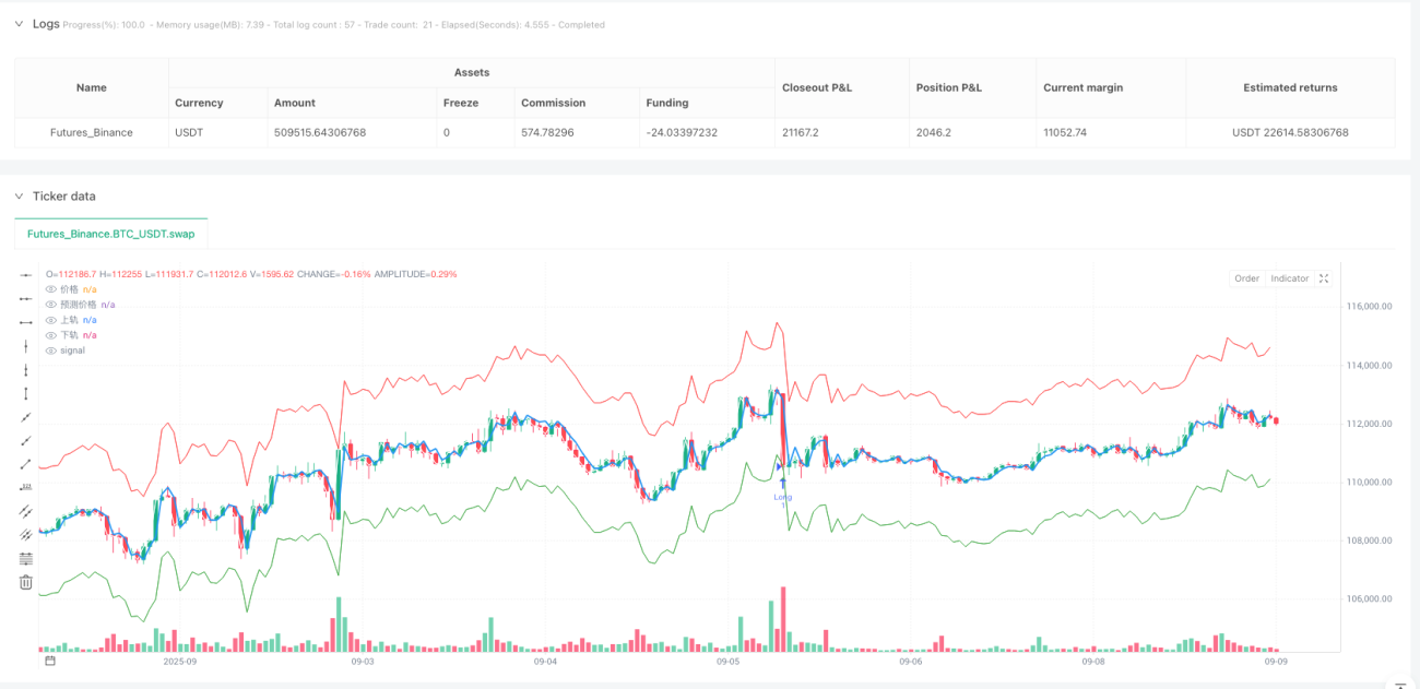
With AR prediction and GARCH volatility estimation, the strategy constructs dynamic confidence intervals:

upperReturnBand = arReturnPredict + stdevFactor * garchStd
lowerReturnBand = arReturnPredict - stdevFactor * garchStd

The trading signal generation logic embodies mean reversion thinking: - Go long when price breaks below the lower band (longSignal = rawPrice < lowerPriceBand) - Go short when price breaks above the upper band (shortSignal = rawPrice > upperPriceBand)

The brilliance of this design lies in the fact that the confidence interval width adjusts dynamically based on market volatility. During high volatility periods, intervals widen, reducing trading frequency; during low volatility periods, intervals narrow, increasing trading opportunities.

What Key Issues Should Be Considered in Practical Application?

1. Model Stability Testing The code includes important stability checks:

if stabilityCheck >= 0.99 or math.abs(phi2) >= 0.99
    scaleFactor = 0.95 / math.max(stabilityCheck, math.abs(phi2) + 0.01)

This ensures AR model stationarity, avoiding divergent prediction results.

2. Parameter Convergence Constraints GARCH models require α + β < 1 to ensure long-term variance existence:

if sumParam >= 0.999
    scale = 0.99 / sumParam

3. Necessity of Filtering Mechanisms The strategy provides RSI filtering options, which are important in practical applications. Pure statistical models might ignore trending characteristics of markets, and the addition of technical indicators can provide additional confirmation signals.

Strategy Limitations and Improvement Directions

Although this strategy is theoretically elegant, practical application still requires consideration of:

Data Frequency Selection: AR-GARCH models perform very differently across various timeframes. High-frequency data provides more information but also introduces more noise.

Parameter Time-Variation: Current implementation assumes AR and GARCH parameters remain constant within the estimation window, but actual market structure may change.

Trading Cost Impact: Statistical arbitrage strategies typically require high trading frequency, making commission and slippage costs significant considerations.

Conclusion: The Value of Statistical Modeling in Quantitative Trading

This AR-GARCH strategy demonstrates the powerful capabilities of modern statistics in financial modeling. It’s not a simple combination of technical indicators, but rather a deep exploration of the statistical properties of financial time series.

For quantitative traders, understanding the value of such strategies lies not only in direct application but also in cultivating the ability to analyze markets with statistical thinking. In today’s era of AI and machine learning dominance, these classical statistical models remain important foundations for understanding markets and constructing strategies.

Strategy source code
/*backtest
start: 2025-04-01 00:00:00
end: 2025-09-09 08:00:00
period: 1h
basePeriod: 1h
exchanges: [{"eid":"Futures_Binance","currency":"BTC_USDT","balance":500000}]
*/

//@version=5
strategy("AR(2)-GARCH Strategy", overlay=true)

//策略参数设置:配置AR模型、GARCH模型和交易信号的各项参数
lengthReg = input.int(50, "AR估计窗口", minval=50, maxval=200);//AR模型回归窗口长度

//GARCH波动率模型参数:控制条件方差的计算
useGarch = input.bool(true, "启用GARCH波动率");//是否启用GARCH波动率建模
garchAlpha = input.float(0.1, "GARCH Alpha", minval=0.01, maxval=0.3, step=0.01);//GARCH模型alpha参数
garchBeta = input.float(0.85, "GARCH Beta", minval=0.5, maxval=0.95, step=0.01);//GARCH模型beta参数

//交易信号生成参数:控制买卖信号的敏感度
stdevFactor = input.float(2.0, "标准差倍数", minval=1.0, maxval=3.0, step=0.1);//交易波段的标准差倍数

//风险控制参数:设置止损止盈水平
stopLossPerc = input.float(2.0, "止损 (%)", minval=0.5, maxval=5.0, step=0.1);//止损百分比
takeProfitPerc = input.float(4.0, "止盈 (%)", minval=1.0, maxval=10.0, step=0.1);//止盈百分比

//RSI过滤器参数:添加技术指标过滤条件
useRsiFilter = input.bool(false, "启用RSI过滤");//是否启用RSI过滤器
rsiLen = input.int(14, "RSI周期", minval=7, maxval=21);//RSI指标计算周期
rsiOB = input.float(70, "RSI超买线", minval=60, maxval=80);//RSI超买阈值
rsiOS = input.float(30, "RSI超卖线", minval=20, maxval=40);//RSI超卖阈值

//数据预处理:计算收益率序列
rawPrice = close;//原始收盘价
returns = math.log(rawPrice / rawPrice[1]);//对数收益率序列

//获取滞后收益率数据:AR(2)模型需要前两期的收益率数据
returns1 = returns[1];//滞后1期的收益率
returns2 = returns[2];//滞后2期的收益率

//计算收益率序列的移动平均值:作为AR模型的均值项
returnsMean = ta.sma(returns, lengthReg);//收益率的简单移动平均

//AR(2)模型系数计算:使用Yule-Walker方程求解自回归系数
//自协方差函数计算:计算不同滞后期的自协方差
calcAutoCovariance(data, lag, length) =>
    mean = ta.sma(data, length);//计算数据的均值
    sum = 0.0;//协方差累计值
    count = 0;//有效数据点计数
    for i = lag to length - 1
        if not na(data[i]) and not na(data[i-lag])
            sum := sum + (data[i] - mean) * (data[i-lag] - mean);//计算协方差分子
            count := count + 1;//累计有效数据点
    count > 0 ? sum / count : 0.0;//返回协方差值

//计算AR(2)模型所需的自协方差:用于Yule-Walker方程
c0 = calcAutoCovariance(returns, 0, lengthReg);//滞后0期的自协方差(即方差)
c1 = calcAutoCovariance(returns, 1, lengthReg);//滞后1期的自协方差
c2 = calcAutoCovariance(returns, 2, lengthReg);//滞后2期的自协方差

//Yule-Walker方程求解:计算AR(2)模型的两个自回归系数
// φ₁ = (c₁c₀ - c₂c₁) / (c₀² - c₁²)
// φ₂ = (c₂c₀ - c₁²) / (c₀² - c₁²)
denominator = c0 * c0 - c1 * c1;//分母计算
phi1 = denominator != 0 ? (c1 * c0 - c2 * c1) / denominator : 0.0;//第一个自回归系数
phi2 = denominator != 0 ? (c2 * c0 - c1 * c1) / denominator : 0.0;//第二个自回归系数

//AR(2)稳定性检验:确保模型稳定性条件 |φ₁| + |φ₂| < 1 且 |φ₂| < 1
stabilityCheck = math.abs(phi1) + math.abs(phi2);//计算系数绝对值之和
if stabilityCheck >= 0.99 or math.abs(phi2) >= 0.99
    scaleFactor = 0.95 / math.max(stabilityCheck, math.abs(phi2) + 0.01);//计算缩放因子
    phi1 := phi1 * scaleFactor;//调整第一个系数
    phi2 := phi2 * scaleFactor;//调整第二个系数

//AR(2)收益率预测:根据历史收益率和AR系数预测下一期收益率
arReturnPredict = returnsMean + phi1 * (returns1 - returnsMean) + phi2 * (returns2 - returnsMean);//AR(2)预测公式

//计算AR模型的预测残差:用于GARCH建模
arResidual = returns - arReturnPredict;//AR模型的预测残差

//GARCH(1,1)波动率建模:对AR残差进行条件方差建模
var float garchVariance = na;//GARCH方差变量
var float longTermVar = na;//长期方差变量

//长期方差初始化:使用历史残差计算初始方差值
if na(longTermVar) and bar_index > lengthReg
    longTermVar := ta.variance(arResidual, lengthReg);//计算长期方差

//GARCH参数调整:确保参数满足收敛条件
adjustedAlpha = garchAlpha;//调整后的alpha参数
adjustedBeta = garchBeta;//调整后的beta参数
sumParam = garchAlpha + garchBeta;//参数和

if sumParam >= 0.999
    scale = 0.99 / sumParam;//计算参数缩放比例
    adjustedAlpha := garchAlpha * scale;//调整alpha参数
    adjustedBeta := garchBeta * scale;//调整beta参数

//GARCH(1,1)递归更新:根据GARCH公式更新条件方差
if useGarch and not na(longTermVar) and not na(arResidual)
    if na(garchVariance)
        garchVariance := longTermVar;//初始化GARCH方差
    else
        omega = (1 - adjustedAlpha - adjustedBeta) * longTermVar;//GARCH常数项
        garchVariance := omega + adjustedAlpha * math.pow(arResidual[1], 2) +  adjustedBeta * garchVariance[1];//GARCH递归公式

//条件标准差计算:从条件方差计算标准差
garchStd = useGarch and not na(garchVariance) ? math.sqrt(math.max(garchVariance, 0.0001)) : ta.stdev(arResidual, 20);//启用GARCH时使用条件标准差,否则使用历史标准差

//收益率空间的置信区间构建:基于AR预测和GARCH波动率
upperReturnBand = arReturnPredict + stdevFactor * garchStd;//上轨:预测收益率加上标准差倍数
lowerReturnBand = arReturnPredict - stdevFactor * garchStd;//下轨:预测收益率减去标准差倍数

//将置信区间转换为价格空间:用于实际交易信号生成
//基于预测收益率计算预测价格
predictedPrice = rawPrice[1] * math.exp(arReturnPredict);//根据预测收益率计算预测价格
upperPriceBand = rawPrice[1] * math.exp(upperReturnBand);//上轨价格
lowerPriceBand = rawPrice[1] * math.exp(lowerReturnBand);//下轨价格

//交易信号生成:基于当前价格相对于置信区间的位置
longSignal = rawPrice < lowerPriceBand;//做多信号:当前价格低于下轨
shortSignal = rawPrice > upperPriceBand;//做空信号:当前价格高于上轨

//RSI过滤器:使用RSI指标过滤交易信号
if useRsiFilter
    rsi = ta.rsi(rawPrice, rsiLen);//计算RSI指标
    longSignal := longSignal and rsi < rsiOS;//做多信号需要RSI超卖确认
    shortSignal := shortSignal and rsi > rsiOB;//做空信号需要RSI超买确认

//策略执行:根据交易信号开仓和平仓
//开仓操作:根据信号建立多头或空头仓位
if longSignal
    strategy.entry("Long", strategy.long);//开多仓

if shortSignal
    strategy.entry("Short", strategy.short);//开空仓

//风险控制:设置止损止盈条件
if strategy.position_size > 0
    strategy.exit("Long Exit", "Long", 
                 stop=strategy.position_avg_price * (1 - stopLossPerc/100),
                 limit=strategy.position_avg_price * (1 + takeProfitPerc/100));//多仓止损止盈

if strategy.position_size < 0
    strategy.exit("Short Exit", "Short",
                 stop=strategy.position_avg_price * (1 + stopLossPerc/100),
                 limit=strategy.position_avg_price * (1 - takeProfitPerc/100));//空仓止损止盈

//图表显示:在图表上绘制价格、预测线和交易信号
//主要价格线和预测线:显示实际价格和基于收益率预测的价格
plot(rawPrice, color=color.white, linewidth=1, title="价格");//绘制实际价格线
plot(predictedPrice, color=color.blue, linewidth=2, title="预测价格");//绘制预测价格线
plot(upperPriceBand, color=color.red, linewidth=1, title="上轨");//绘制上轨线
plot(lowerPriceBand, color=color.green, linewidth=1, title="下轨");//绘制下轨线

//交易信号标记:在图表上标记买卖信号点
plotshape(longSignal, style=shape.triangleup, location=location.belowbar, 
         color=color.green, size=size.small, title="买入");//标记买入信号
plotshape(shortSignal, style=shape.triangledown, location=location.abovebar, 
         color=color.red, size=size.small, title="卖出");//标记卖出信号