BBP Adaptive Distribution Strategy

Overview
This strategy is an innovative quantitative trading system based on statistical distribution theory, combining the traditional Bull Bear Power (BBP) indicator with adaptive distribution fitting techniques. The core innovation lies in breaking away from the fixed normal distribution assumption of traditional technical analysis. By calculating high-order statistical characteristics (skewness and kurtosis) of market data in real-time, it dynamically adjusts trading thresholds to align signal generation with the market's true distribution features. The strategy is equipped with a three-level dynamic take-profit system based on ATR and market condition assessment, achieving precise adaptation to different market environments. It is particularly suitable for cryptocurrency markets with distinct distribution characteristics, effectively identifying statistically significant anomalies and avoiding false signals caused by incorrect distribution assumptions.
Strategy Principles
The core operational mechanism includes the following key components:
-
BBP Indicator Calculation: Constructs a fundamental indicator reflecting market bull-bear force comparison by calculating the sum of the difference between high price and EMA (bull power) and the difference between low price and EMA (bear power). Positive values indicate bullish dominance, while negative values indicate bearish dominance.
-
Distribution Characteristic Analysis: Employs high-order moment calculation methods to perform statistical analysis on the BBP sequence, outputting four key statistics: mean, standard deviation, skewness (third-order central moment), and excess kurtosis (fourth-order central moment minus 3), comprehensively depicting the distribution shape of market data. Skewness reflects distribution asymmetry, while kurtosis reflects tail thickness and extreme event frequency.
-
Adaptive Threshold Generation:
- Calculates standard normal quantile as baseline Z-value based on significance level
- Applies t-distribution approximation correction when excess kurtosis exceeds threshold, deriving degrees of freedom from kurtosis and expanding tolerance range
- Applies Cornish-Fisher expansion for asymmetry correction when skewness exceeds threshold
- Generates upper and lower threshold lines dynamically adjusted according to market's true distribution characteristics
-
Market Condition Assessment:
- Volume dimension: Quantifies market participation into high, medium, and low levels through the ratio of current volume to period average
- Price position dimension: Locates price's relative position in historical range through percentile ranking algorithm
- Composite scoring mechanism: Averages scores from both dimensions to form take-profit adjustment coefficient
-
Dynamic Take-Profit System:
- Adopts three-level take-profit design with multipliers based on golden ratio (1.618, 2.382, 3.618)
- Each take-profit level distance = ATR × fixed multiplier × dynamic adjustment coefficient
- Expands take-profit targets in strong trends with high volume and high percentiles, tightens take-profit distance in low participation scenarios
-
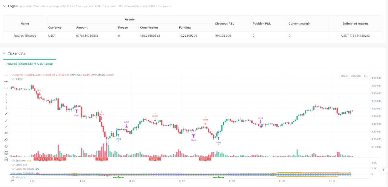
Signal Generation and Execution:
- Long signal: Opens long when BBP crosses above adaptive upper threshold
- Short signal: Opens short when BBP crosses below adaptive lower threshold
- Exit signal: Closes position when BBP reverts to mean line, following mean reversion principle
Strategy Advantages
-
Solid Statistical Theory Foundation: Breaks away from traditional strategies' fixed normal distribution assumption, dynamically adjusting decision criteria based on market's true distribution characteristics. Reconstructs signal generation logic from a statistical perspective with rigorous theoretical support.
-
Outstanding Adaptive Capability: Through real-time monitoring of skewness and kurtosis, the strategy automatically identifies changes in market distribution characteristics. Raises upper threshold in positively skewed markets to avoid chasing highs, expands threshold range in fat-tailed markets to avoid overreacting to normal fluctuations, truly achieving "strategy adapts to market."
-
Multi-Dimensional Comprehensive Assessment: Combines three dimensions - price momentum, volume activity, and price relative position - to construct a comprehensive market condition assessment system, avoiding one-dimensional judgment bias.
-
Dynamic Risk Management: Three-level take-profit system with dynamic adjustment mechanism adaptively optimizes take-profit distances based on market heat. Fully captures profit space in trending markets while quickly realizing gains in weak markets.
-
High Signal Quality: Through statistical significance testing, triggers trades only at true distribution anomalies, effectively reducing false signal rate and improving statistical validity of trades.
-
Intuitive Visualization: Through dynamic threshold lines, standard deviation reference lines, and signal markers, clearly displays the strategy's adaptive adjustment process, facilitating understanding and monitoring.
Strategy Risks
-
High Parameter Optimization Complexity: The strategy contains multiple parameters (significance level, skewness threshold, kurtosis threshold, take-profit multipliers, etc.). Optimal parameter combinations vary significantly across different market environments, requiring systematic parameter optimization and backtesting validation.
-
Lack of Clear Stop-Loss Mechanism: The strategy primarily relies on mean reversion exits, lacking hard stop-loss based on price or ATR. In extreme trending markets, if BBP continues to deviate from mean without reverting, it may cause significant unrealized losses and capital tie-up.
-
Poor Adaptability in Ranging Markets: In prolonged narrow-range consolidation, BBP values hover around the mean, difficult to reach adaptive thresholds, resulting in scarce trading opportunities and limited strategy performance.
-
Strong Data Dependency: Distribution characteristic analysis requires sufficient historical data to obtain stable and reliable statistical results. For newly listed coins or instruments with insufficient data, statistics may be unstable in early usage, affecting strategy performance.
-
High Computational Complexity: Real-time calculation of high-order moments, percentile rankings, and dynamic thresholds requires traversing historical data, potentially facing performance bottlenecks in resource-constrained trading environments.
-
Extreme Market Risk: In extreme rapid one-directional moves like flash crashes or surges, BBP may instantly break through thresholds and quickly revert, leading to suboptimal entry points or missed optimal timing.
Optimization Directions
-
Introduce Dynamic Stop-Loss Mechanism:
- ATR-based trailing stop-loss with distance dynamically adjusted based on holding time and profit status
- Technical stop-loss incorporating support and resistance levels
- Adaptive stop-loss based on Maximum Adverse Excursion (MAE)
-
Enhanced Market Environment Recognition:
- Introduce trend strength filter (e.g., ADX), suspending trades when no clear trend exists
- Add volatility state classification to identify and avoid extreme volatility periods
- Incorporate market microstructure indicators to preemptively identify liquidity exhaustion states
-
Parameter Adaptive Optimization:
- Apply rolling window backtesting to dynamically adjust analysis period length
- Introduce machine learning methods (e.g., genetic algorithms, particle swarm optimization) for parameter optimization
- Implement parameter switching mechanism based on market states
-
Signal Quality Enhancement:
- Add volume confirmation condition requiring signal triggers to be accompanied by volume expansion
- Incorporate key technical levels (e.g., previous highs/lows, Fibonacci retracements) for multiple confirmations
- Introduce signal strength scoring system to adjust position size based on score
-
Position Management Optimization:
- Dynamic position allocation based on Kelly Criterion
- Adjust opening ratio according to signal strength and market condition scores
- Implement pyramid scaling in/out strategies
-
Multi-Timeframe Integration:
- Determine major trend direction on higher timeframes, trading only with the trend
- Seek precise entry points on lower timeframes
- Build multi-period resonance confirmation mechanism
Summary
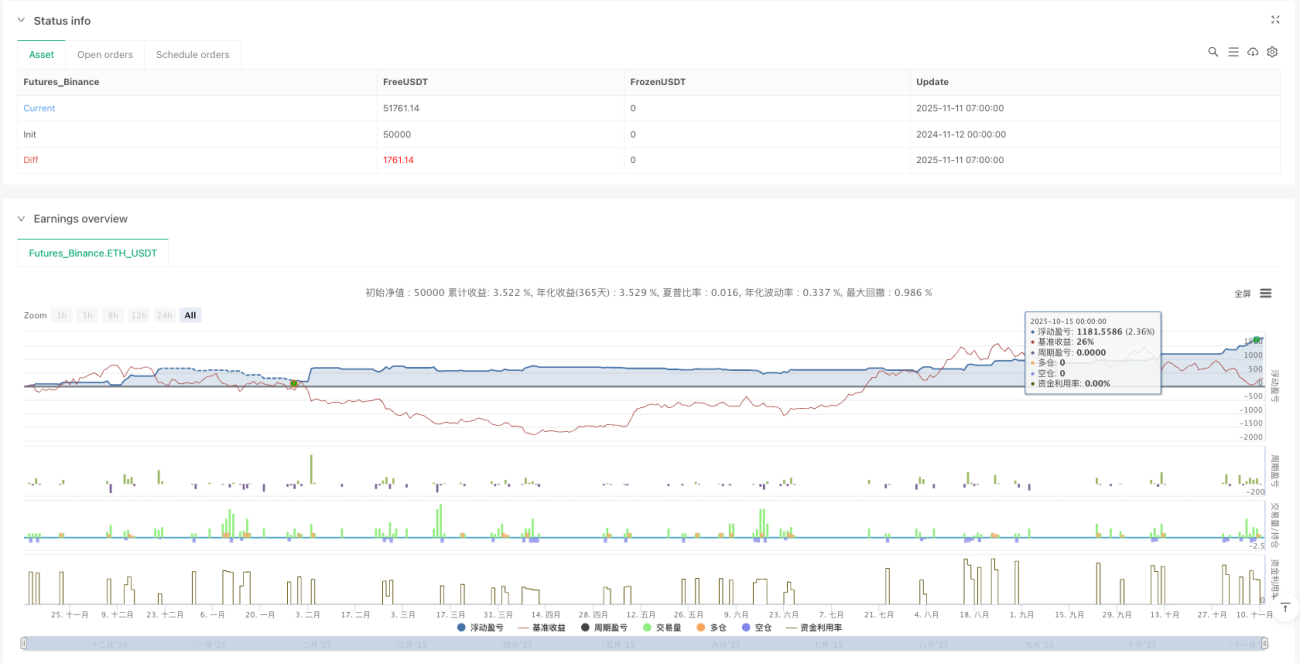
The BBP Adaptive Distribution Strategy represents an innovative attempt at combining technical analysis with modern statistics, fundamentally solving traditional strategies' dependence on normal distribution assumptions through adaptive distribution fitting techniques. The strategy's core value lies in its theoretical innovation and respect for market's true distribution characteristics, maintaining reasonable signal quality across markets with different distribution shapes. The three-level dynamic take-profit system further enhances the strategy's practicality, achieving a good balance between returns and risk.
However, the strategy also has obvious room for improvement. The lack of a clear stop-loss mechanism is the biggest shortcoming and needs priority supplementation in practical application. The complexity of parameter optimization and adaptability issues in ranging markets also need to be addressed by introducing market environment recognition and parameter adaptive mechanisms.
For quantitative traders pursuing theoretical depth and willing to conduct in-depth research, this strategy provides an excellent learning and improvement framework. Recommendations before live trading:
- Conduct thorough historical backtesting and parameter optimization for specific trading instruments
- Add hard stop-loss protection based on ATR or percentage
- Combine with trend filters to avoid trading in unfavorable market environments
- Start with small positions and gradually validate strategy performance in live trading
Overall, this is an innovative strategy with solid theoretical foundation, rigorous design logic, and high research and application value, worthy of in-depth exploration and continuous optimization by quantitative traders.
//@version=5
strategy("BBP Adaptive Distribution Strategy [presentTrading]")

//========================================
// BBP策略参数设置
//========================================
lengthInput = input.int(20, "EMA Length");//EMA周期长度
zLength = input.int(150, "Distribution Analysis Period");//分布分析周期

//自适应分布参数组
dist_group = "Distribution Fitting";
//统计显著性水平,0.05表示95%置信度- 1