En la carga de los recursos... Cargando...

Estrategia de indicadores de impulso de IOR/IFM basada en la teoría de Dow

El autor:¿ Qué pasa?, Fecha: 2023-12-12 17:54:58
Las etiquetas:

Resumen general

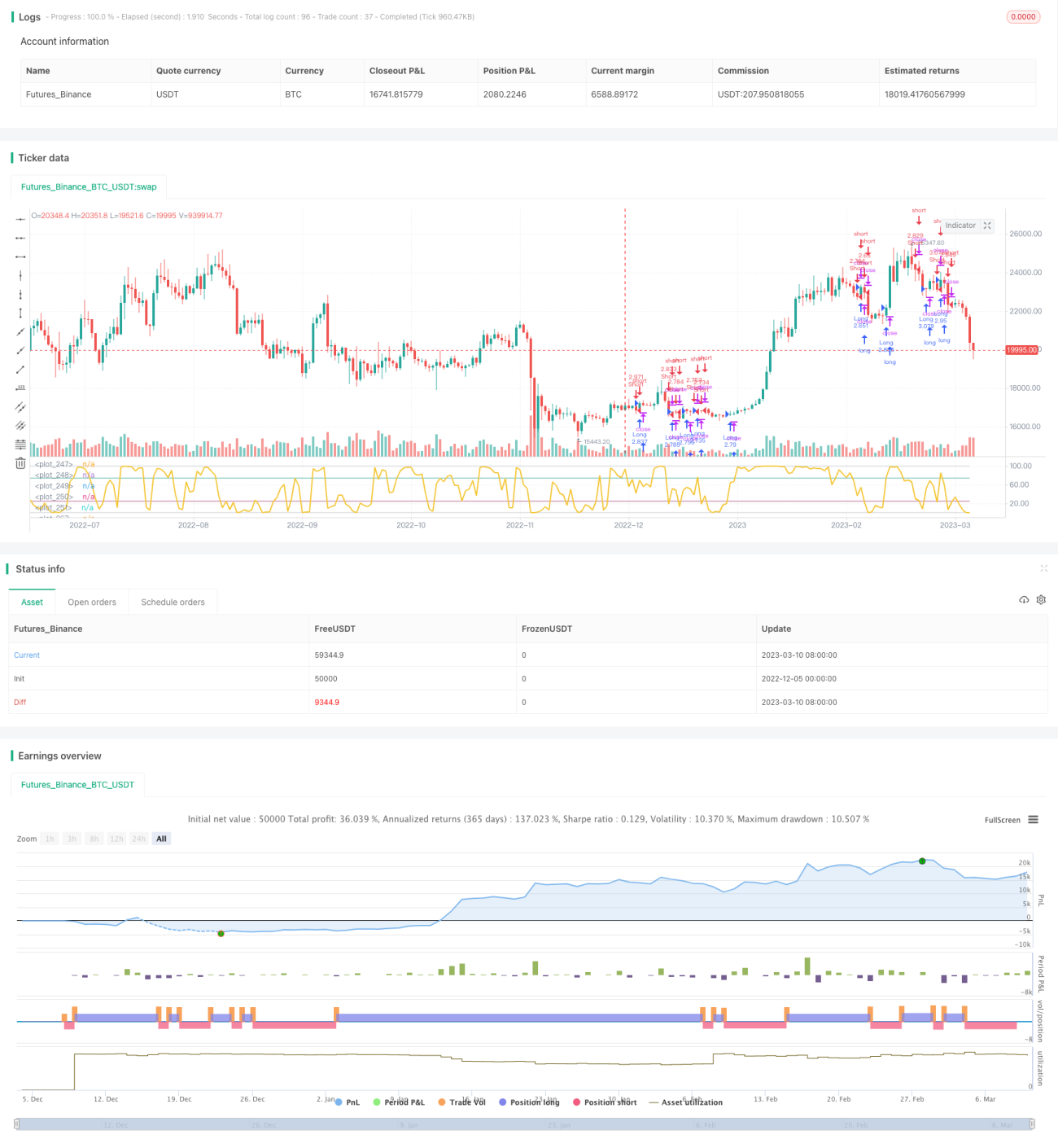
Esta estrategia utiliza el Índice de Fuerza Relativa (RSI) o el Índice de Flujo de Dinero (IFM) para juzgar si el mercado es alcista o bajista, combinado con el coeficiente alcista-bajista de la Teoría Dow para calcular la distribución de probabilidad ajustada.

Principio de la estrategia

Calcular el índice de rentabilidad o la IFM para juzgar el estado actual del mercado (bull o bear)
Cálcule el coeficiente toro-oso de la teoría Dow para reflejar la correlación entre el precio actual y el volumen
Ajustar la distribución de probabilidad del IOR/IFM para determinar una distribución precisa de largo/cortito
Decidir si introducir en función de la sesión actualId y la probabilidad
Pérdida de parada cuando se toma ganancia o se comercializa lateralmente

Análisis de ventajas

Un juicio más preciso del tipo de mercado combinado con la teoría Dow
Considere el factor lateral para evitar la entrada a ciegas
Alta relación riesgo-rendimiento y bajo aprovechamiento

Análisis de riesgos

Pueden ocurrir múltiples errores de juicio con parámetros incorrectos
Se necesitan datos históricos suficientes para apoyar
La lógica de stop loss simple no puede optimizarse para situaciones especiales de mercado

Dirección de optimización

Considere combinar más indicadores para juzgar la sesión de mercado
Añadir una lógica de stop loss más rigurosa basada en la volatilidad, los datos históricos, etc.
Pruebe el aprendizaje automático, etc. para determinar mejores parámetros.

Resumen de las actividades

El resultado general de la prueba de retroceso de esta estrategia es bueno y tiene cierto valor práctico. Pero aún se necesitan más pruebas y ajustes, especialmente para la lógica de stop loss. Funciona mejor como un indicador de juicio de asistencia, no se puede seguir a ciegas.

/*backtest
start: 2022-12-05 00:00:00
end: 2023-03-11 00:00:00
period: 1d
basePeriod: 1h
exchanges: [{"eid":"Futures_Binance","currency":"BTC_USDT"}]
*/

//@version=4

//MIT License

//Copyright (c) 2019 user-Noldo

//Permission is hereby granted, free of charge, to any person obtaining a copy
//of this software and associated documentation files (the "Software"), to deal
//in the Software without restriction, including without limitation the rights
//to use, copy, modify, merge, publish, distribute, sublicense, and/or sell
//copies of the Software, and to permit persons to whom the Software is
//furnished to do so, subject to the following conditions:

//The above copyright notice and this permission notice shall be included in all
//copies or substantial portions of the Software.

//THE SOFTWARE IS PROVIDED "AS IS", WITHOUT WARRANTY OF ANY KIND, EXPRESS OR
//IMPLIED, INCLUDING BUT NOT LIMITED TO THE WARRANTIES OF MERCHANTABILITY,
//FITNESS FOR A PARTICULAR PURPOSE AND NONINFRINGEMENT. IN NO EVENT SHALL THE
//AUTHORS OR COPYRIGHT HOLDERS BE LIABLE FOR ANY CLAIM, DAMAGES OR OTHER
//LIABILITY, WHETHER IN AN ACTION OF CONTRACT, TORT OR OTHERWISE, ARISING FROM,
//OUT OF OR IN CONNECTION WITH THE SOFTWARE OR THE USE OR OTHER DEALINGS IN THE
//SOFTWARE.


strategy("Dow Factor RSI/MFI and Dependent Variable Odd Generator Strategy",shorttitle = "Dow_Factor RSI/MFI & DVOG Strategy", overlay = false, default_qty_type=strategy.percent_of_equity,commission_type=strategy.commission.percent, commission_value=0.125, default_qty_value=100 )
src = close 
lights          = input(title="Barcolor I / 0 ? ", options=["ON", "OFF"], defval="OFF")
method          = input(title="METHOD", options=["MFI", "RSI"], defval="RSI")

length = input(5, minval=2,maxval = 14, title = "Strategy Period")

// Essential Functions 

// Function Sum 

f_sum(_src , _length) => 

    _output  = 0.00 
    
    _length_adjusted = _length < 1 ? 1 : _length
    
    for i = 0 to _length_adjusted-1
        _output := _output + _src[i]


f_sma(_src, _length)=>
    _length_adjusted = _length < 1 ? 1 : _length
    float _sum = 0
    for _i = 0 to (_length_adjusted - 1)
        _sum := _sum + _src[_i]
    _return = _sum / _length_adjusted
   

// Unlocked Exponential Moving Average Function

f_ema(_src, _length)=>
    _length_adjusted = _length < 1 ? 1 : _length
    _multiplier = 2 / (_length_adjusted + 1)
    _return  = 0.00
    _return := na(_return[1]) ? _src : ((_src - _return[1]) * _multiplier) + _return[1]


// Function Standard Deviation

f_stdev(_src,_length) =>

    float _output = na 
    _length_adjusted = _length < 2 ? 2 : _length
    _avg  = f_ema(_src , _length_adjusted)
    evar  = (_src - _avg) * (_src - _avg)
    evar2 = ((f_sum(evar,_length_adjusted))/_length_adjusted)
    
    _output := sqrt(evar2)


// Linear Regression Channels : 

f_pearson_corr(_src1, _src2, _length) =>

    _length_adjusted = _length < 2 ? 2 : _length
    _ema1 = f_ema(_src1, _length_adjusted)
    _ema2 = f_ema(_src2, _length_adjusted)
    isum = 0.0
    for i = 0 to _length_adjusted - 1
        isum := isum + (_src1[i] - _ema1) * (_src2[i] - _ema2)
    isumsq1 = 0.0
    for i = 0 to _length_adjusted - 1
        isumsq1 := isumsq1 + pow(_src1[i] - _ema1, 2)
    isumsq2 = 0.0
    for i = 0 to _length_adjusted - 1
        isumsq2 := isumsq2 + pow(_src2[i] - _ema2, 2)
    pcc = isum/(sqrt(isumsq1*isumsq2))
    pcc


// Dow Theory Cycles 


dow_coeff = f_pearson_corr(src,volume,length)

dow_bull_factor = (1 + dow_coeff)
dow_bear_factor = (1 - dow_coeff)


// MONEY FLOW INDEX =====> FOR BULL OR BEAR MARKET (CLOSE)


upper_s = f_sum(volume * (change(src) <= 0 ? 0 : src), length)
lower_s = f_sum(volume * (change(src) >= 0 ? 0 : src), length)

_market_index = rsi(upper_s, lower_s)


// RSI (Close)

// Function RMA 

f_rma(_src, _length) =>
    _length_adjusted = _length < 1 ? 1 : _length
    alpha = _length_adjusted
    sum = 0.0
    sum := (_src + (alpha - 1) * nz(sum[1])) / alpha


// Function Relative Strength Index (RSI)

f_rsi(_src, _length) => 

    _output = 0.00 
    _length_adjusted = _length < 0 ? 0 : _length

    u = _length_adjusted < 1 ? max(_src - _src[_length_adjusted], 0) : max(_src - _src[1] , 0) // upward change
    d = _length_adjusted < 1 ? max(_src[_length_adjusted] - _src, 0) : max(_src[1] - _src , 0) // downward change
    rs = f_rma(u, _length) / f_rma(d, _length)
    res = 100 - 100 / (1 + rs)
    res


_rsi = f_rsi(src, length)


// Switchable Method Codes 

_method = 0.00 


if (method=="MFI")

    _method:= _market_index 
    
if (method=="RSI")

    _method:= _rsi   
    


// Conditions  

_bull_gross  = (_method )
_bear_gross  = (100 - _method )

_price_stagnant = ((_bull_gross * _bear_gross ) / 100)
_price_bull     =  (_bull_gross - _price_stagnant) 
_price_bear     =  (_bear_gross - _price_stagnant) 


_coeff_price = (_price_stagnant + _price_bull + _price_bear) / 100 

_bull     = _price_bull / _coeff_price 
_bear     = _price_bear / _coeff_price 
_stagnant = _price_stagnant / _coeff_price



// Market Types with Dow Factor

_temp_bull_gross     =  _bull     * dow_bull_factor       

_temp_bear_gross     =  _bear     * dow_bear_factor 


// Addition : Odds with Stagnant Market 


_coeff_normal = (_temp_bull_gross + _temp_bear_gross) / 100


// ********* OUR RSI / MFI VALUE ***********

_value        = _temp_bull_gross / _coeff_normal


// Temporary Pure Odds 

_temp_stagnant = ((_temp_bull_gross * _temp_bear_gross) / 100)
_temp_bull     = _temp_bull_gross - _temp_stagnant 
_temp_bear     = _temp_bear_gross - _temp_stagnant 


// Now we ll do venn scheme (Probability Cluster)
// Pure Bull + Pure Bear + Pure Stagnant = 100 
// Markets will get their share in the Probability Cluster 

 
_coeff = (_temp_stagnant + _temp_bull + _temp_bear) / 100

_odd_bull     = _temp_bull / _coeff
_odd_bear     = _temp_bear / _coeff
_odd_stagnant = _temp_stagnant / _coeff


_positive_condition     = crossover (_value,50)
_negative_condition     = crossunder(_value,50)
_stationary_condition   = ((_odd_stagnant > _odd_bull ) and (_odd_stagnant > _odd_bear))


// Strategy 

closePosition = _stationary_condition


if (_positive_condition)
    strategy.entry("Long", strategy.long, comment="Long")
    
strategy.close(id = "Long", when = closePosition )

if (_negative_condition)
    strategy.entry("Short", strategy.short, comment="Short")
    
strategy.close(id = "Short", when = closePosition )    


// Plot Data

// Plotage 

oversold   = input(25 , type = input.integer , title = "Oversold")   
overbought = input(75 , type = input.integer , title = "Overbought") 

zero    = 0 
hundred = 100
limit   = 50

// Plot Data 

stagline       = hline(limit      , color=color.new(color.white,0)   , linewidth=1, editable=false)
zeroline       = hline(zero       , color=color.new(color.silver,100), linewidth=0, editable=false)
hundredline    = hline(hundred    , color=color.new(color.silver,100), linewidth=0, editable=false)
oversoldline   = hline(oversold   , color=color.new(color.silver,100), linewidth=0, editable=false)
overboughtline = hline(overbought , color=color.new(color.silver,100), linewidth=0, editable=false)

// Filling Borders

fill(zeroline       , oversoldline   , color=color.maroon  , transp=88 , title = "Oversold Area")
fill(oversoldline   , stagline       , color=color.red     , transp=80 , title = "Bear Market")
fill(stagline       , overboughtline , color=color.green   , transp=80 , title = "Bull Market")
fill(overboughtline , hundredline    , color=color.teal    , transp=88 , title = "Overbought Market")


// Plot DOW Factor Methods

plot(_value, color = #F4C430 , linewidth = 2 , title = "DOW F-RSI" , transp = 0)

// Plot border lines

plot(oversold  ,style = plot.style_line,color = color.new(color.maroon,30),linewidth = 1)
plot(overbought,style = plot.style_line,color = color.new(color.teal,30)  ,linewidth = 1)


plot(zero     ,style = plot.style_line , color = color.new(color.silver,30) , linewidth = 1 ,editable = false)
plot(hundred  ,style = plot.style_line , color = color.new(color.silver,30) , linewidth = 1 ,editable = false)


// Switchable Barcolor ( On / Off)

_lights = 0.00 


if (lights=="ON")

    _lights:= 1.00
    
if (lights=="OFF")

    _lights:= -1.00   


bcolor_on  = _lights ==  1.00
bcolor_off = _lights == -1.00


barcolor((_positive_condition and bcolor_on)    ? color.green : (_negative_condition and bcolor_on) ? color.red : 
          (_stationary_condition and bcolor_on) ? color.yellow : na)


// Alerts 

alertcondition(_positive_condition , title='Strong Buy !', message='Strong Buy Signal ')
alertcondition(crossover(_value,overbought) , title='Gradual Buy', message='Gradual Buy Signal')
alertcondition(crossover(_value,oversold)   , title='Gradual Buy', message='Gradual Buy Signal')

alertcondition(crossunder(_value,overbought) , title='Gradual Sell', message='Gradual Sell Signal')
alertcondition(crossunder(_value,oversold)   , title='Gradual Sell', message='Gradual Sell Signal')

alertcondition(_negative_condition , title='Strong Sell !', message='Strong Sell Signal ')

Más.