Estrategia de reversión a la media de banda de Bollinger basada en el costo del dólar

Descripción general
La estrategia es una estrategia de inversión inteligente que combina la ley del promedio de costos en dólares (DCA) y los indicadores técnicos de la banda de Brin. Se invierte utilizando el principio de la regresión de la mediana, construyendo sistemáticamente una posición durante la corrección de precios. El núcleo de la estrategia es realizar operaciones de compra de una cantidad fija cuando el precio cae por debajo de la banda de Brin, lo que permite obtener un mejor precio de entrada durante los períodos de ajuste del mercado.
Principio de estrategia
El principio central de la estrategia se basa en tres fundamentos: 1) el promedio de costos en dólares, que reduce el riesgo al momento de elegir invertir una cantidad fija periódicamente; 2) la teoría de la regresión a la media, que considera que los precios finalmente regresarán a sus niveles promedio históricos; 3) el indicador de la banda de Brin, que se utiliza para identificar las zonas de sobreventa y sobreventa. Cuando los precios rompen la banda de Brin, se activa una señal de compra.
Ventajas estratégicas
- Reducir el riesgo de error humano a través de la compra sistemática en lugar de un juicio subjetivo
- Aprovechar las oportunidades de reajuste - ejecutar automáticamente la operación de compra cuando el precio supera la caída
- Ajuste de parámetros flexibles - los parámetros de la banda de Bryn y el monto de la inversión se pueden ajustar según las diferentes condiciones del mercado
- Reglas claras de entrada y salida - señales objetivas basadas en indicadores técnicos
- Ejecución automatizada - sin intervención humana y evitando transacciones emocionales
Riesgo estratégico
- Riesgo de fallo de la regresión a la media - puede generar más señales falsas en un mercado de tendencia
- Riesgo de gestión de fondos - Necesidad de reservar fondos suficientes para responder a las señales de compra en serie
- Riesgo de optimización de parámetros: la optimización excesiva puede hacer que la estrategia no funcione
- Dependencia del entorno del mercado - puede tener un rendimiento deficiente en mercados con gran volatilidad
Se recomienda la adopción de un sistema de gestión de fondos estricto y la evaluación periódica del rendimiento de la estrategia para administrar estos riesgos.
Dirección de optimización de la estrategia
- Introducción de filtros de tendencia para evitar operaciones de reversión en una tendencia fuerte
- Mecanismo de confirmación de múltiples períodos de tiempo
- Optimizar el sistema de gestión de fondos y ajustar el monto de las inversiones en función de la fluctuación de la tasa
- Se añade el mecanismo de cierre de ganancias, que se cierra cuando el precio regresa a la media
- Considerar la combinación de otros indicadores técnicos para mejorar la fiabilidad de la señal
Resumir
Es una estrategia robusta que combina análisis técnico con métodos de inversión sistematizados. Se trata de una estrategia robusta que combina el análisis técnico con métodos de inversión sistematizados. Se trata de una estrategia robusta que combina el análisis técnico con métodos de inversión sistematizados. Se trata de una estrategia robusta que combina el análisis técnico con métodos de inversión sistematizados.
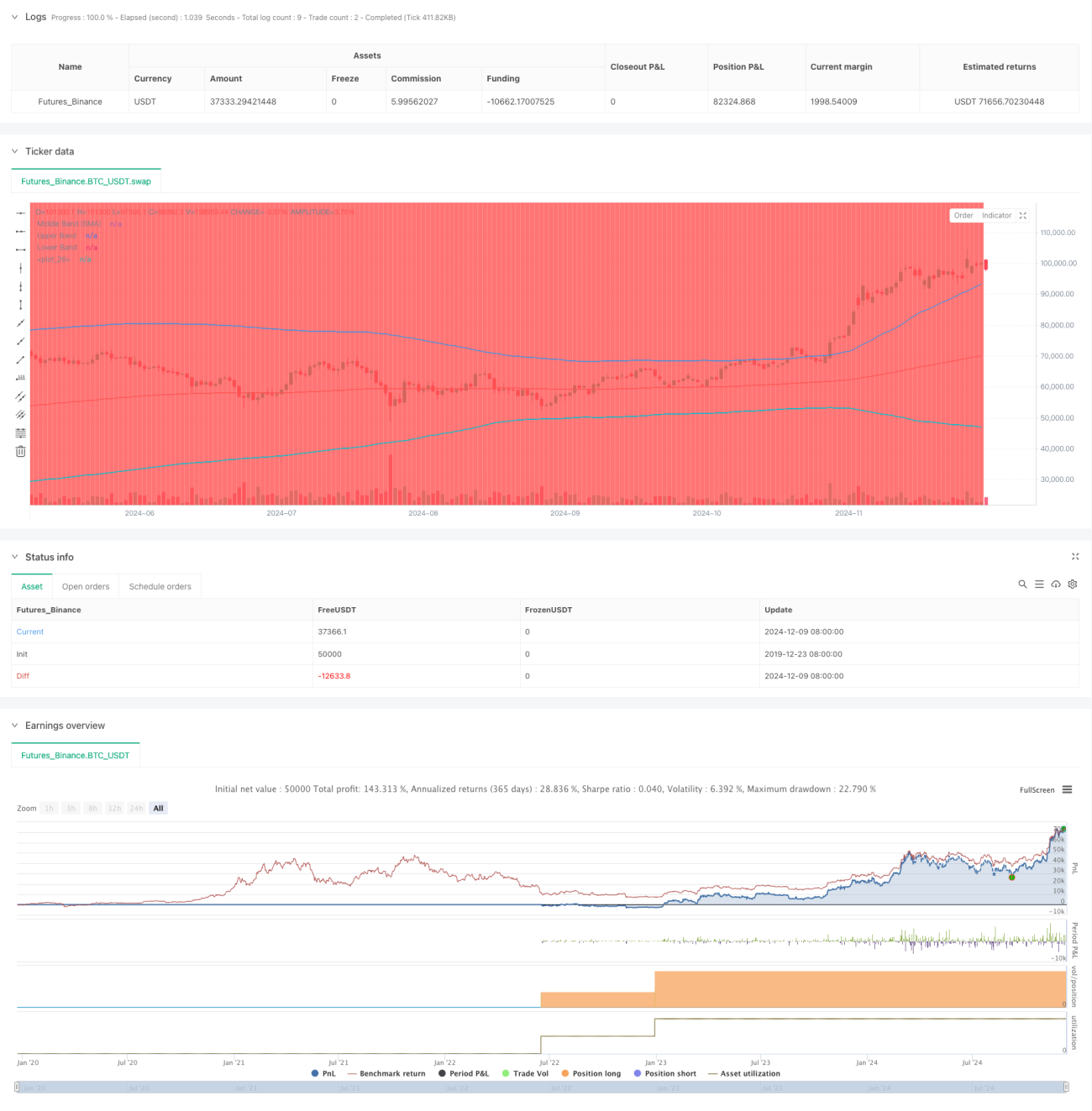
/*backtest
start: 2019-12-23 08:00:00
end: 2024-12-10 08:00:00
period: 1d
basePeriod: 1d
exchanges: [{"eid":"Futures_Binance","currency":"BTC_USDT"}]
*/

//@version=5
strategy("DCA Strategy with Mean Reversion and Bollinger Band", overlay=true) // Define the strategy name and set overlay=true to display on the main chart

// Inputs for investment amount and dates- 1