Estrategia de trading de momentum multidimensional basada en análisis de espectro cuántico

Descripción general
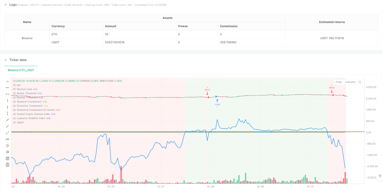
La estrategia es un innovador sistema de comercio cuantitativo que combina los principios de la mecánica cuántica, la estadística y la economía. Construye un marco integral de análisis de mercado mediante la combinación de la media móvil simple (SMA), el análisis estadístico de Z-Score, el componente de fluctuación cuántica, el indicador de dinámica económica y el índice de estabilidad de Lyapunov.
Principio de estrategia
La estrategia se basa en cinco pilares tecnológicos principales:
- El módulo de análisis estadístico utiliza el SMA y la diferencia estándar para calcular el Z-Score, que evalúa la posición relativa de los precios.
- El componente cuántico convierte el Z-Score en un oscilador que simula las propiedades de oscilación del estado cuántico a través de la función exponencial y la función de la sincronía.
- El componente económico mide la dinámica del mercado con el uso de la relación entre el EMA rápido y lento.
- El índice de Lyapunov evalúa el estado del mercado mediante el análisis de la estabilidad combinada de los componentes cuánticos y económicos.
- El índice de perspectivas de mercado integral (COI) integra todos los componentes con diferentes pesos para formar la señal de negociación final.
Ventajas estratégicas
- El análisis multidimensional proporciona una visión más completa del mercado, reduciendo el desvío que un solo indicador puede generar.
- La introducción de los componentes cuánticos ofrece una perspectiva única de las fluctuaciones del mercado que ayuda a capturar oportunidades a corto plazo.
- La aplicación del Índice de Lyapunov es una evaluación eficaz de la estabilidad del mercado y mejora la capacidad de gestión de riesgos.
- El diseño de peso ajustable permite que las estrategias se adapten con flexibilidad a diferentes circunstancias del mercado.
- El diseño de la línea neutral del índice integral proporciona un límite claro de la señal de negociación.
Riesgo estratégico
- La multiplicación de indicadores puede causar un retraso en la señal y afectar el tiempo de entrada.
- La optimización excesiva de los parámetros puede conducir a un riesgo de sobreajuste.
- En un mercado de alta volatilidad, los componentes cuánticos pueden generar señales demasiado frecuentes.
- Los componentes económicos pueden generar señales engañosas en el mercado horizontal.
- El riesgo debe ser controlado mediante la fijación de un stop loss razonable.
Dirección de optimización de la estrategia
- Introducción de un sistema de peso adaptativo para ajustar el peso de los componentes según la dinámica del entorno del mercado.
- Aumentar el filtro de frecuencia de oscilación para ajustar la sensibilidad de la señal durante las altas oscilaciones.
- La integración de los indicadores de sentimiento del mercado proporciona señales de confirmación adicionales.
- Desarrollar mecanismos dinámicos de stop loss para ajustar los niveles de stop loss según las condiciones del mercado.
- Añade un filtro de tiempo para evitar abrir una posición en un momento desfavorable.
Resumir
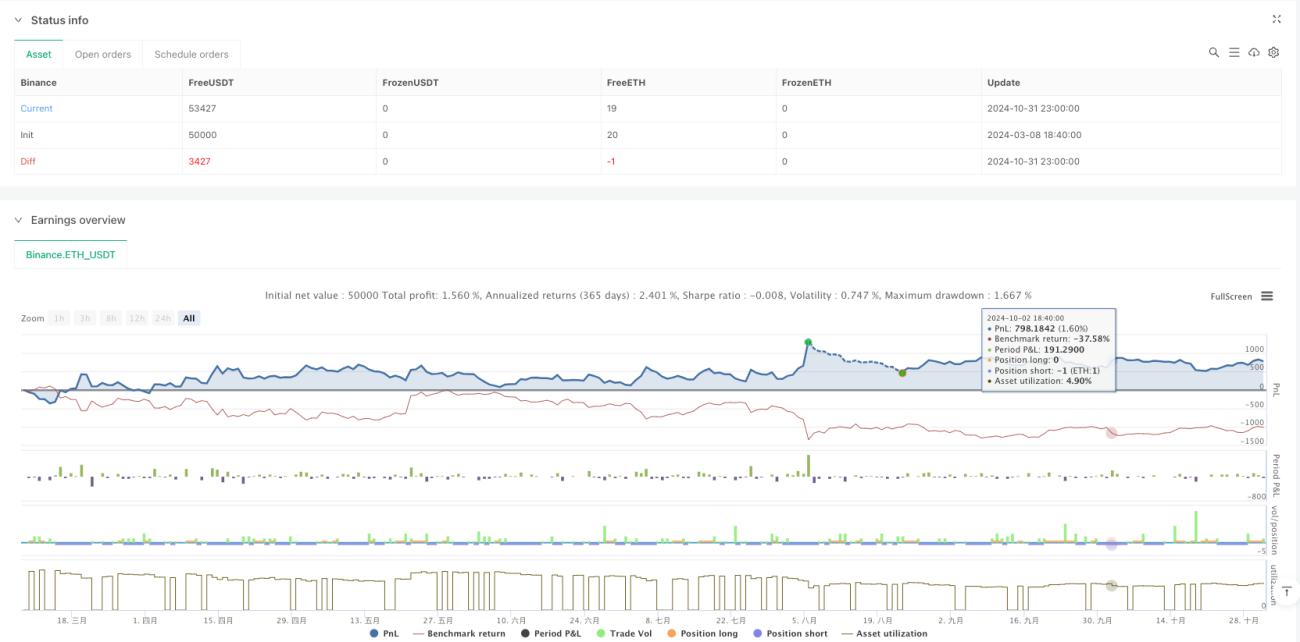
Se trata de una innovadora estrategia de trading cuantitativo que construye un marco integral de análisis de mercado mediante la fusión de teorías multidisciplinarias. Aunque hay algunos lugares que necesitan ser optimizados, su método de análisis multidimensional ofrece una perspectiva única para la toma de decisiones de trading. A través de la optimización continua y la mejora de la gestión de riesgos, la estrategia espera mantener un rendimiento estable en diferentes entornos de mercado.
- 1