Estrategia de análisis de tendencias estadísticas multibanda

BB SMA EMA SD PL QB
Fecha de creación: 2025-02-20 16:45:59 Última modificación: 2025-02-20 16:45:59
Copiar: 1 Número de Visitas: 348
2
Seguir
319
Seguidores

Estrategia de análisis de tendencias estadísticas multibanda Estrategia de análisis de tendencias estadísticas multibanda

Descripción general

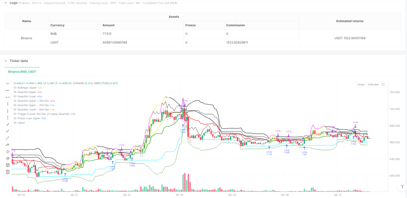
Se trata de una estrategia de negociación basada en el análisis de múltiples bandas estadísticas y tendencias. La estrategia combina el uso de bandas de Brin, bandas de parámetros y la ley de la brecha para identificar las áreas clave de soporte / resistencia, y utiliza la diferencia estándar inferior de las bandas de parámetros superiores como señal de activación para determinar el momento de entrada y salida.

Principio de estrategia

El principio central de la estrategia es capturar las tendencias del mercado a través de la intersección de múltiples bandas estadísticas. La estrategia contiene principalmente los siguientes componentes clave:

  1. El sistema de bandas de Brin - utilizado para determinar el rango de fluctuación de los precios, se convierte en una alerta amarilla cuando los precios se desvian.
  2. Sistema de bandas de dígitos - para calcular los dígitos superiores y inferiores de los precios, y para evaluar la probabilidad de los valores máximos de los precios.
  3. El sistema de bandas rectangulares - que calcula el nivel de significancia basado en los retornos históricos - se usa para medir el exceso de compra y venta.
  4. Sistema de activación - la línea de diferencia estándar inferior de la franja de dígitos superior es la señal de activación principal, y el precio se mantiene por encima de esta línea como una señal de avance.
  5. Sistema de confirmación - Filtra las señales falsas mediante la configuración de un número de líneas K de confirmación en serie.

Ventajas estratégicas

  1. La estabilidad de la señal es alta - el uso superpuesto de múltiples bandas estadísticas puede reducir eficazmente las señales falsas.
  2. Adaptabilidad - Las estrategias pueden adaptarse a diferentes períodos de tiempo y condiciones de mercado.
  3. Control de riesgos perfecto - Dividir las zonas de riesgo con múltiples estadísticas y un mecanismo de deterioro.
  4. Flexibilidad de parámetros - Ofrece una gran variedad de opciones de parámetros que se pueden optimizar según las diferentes características del mercado.
  5. Visualización clara: las líneas de los indicadores son claramente distinguidas en color y las señales de negociación son intuitivas.

Riesgo estratégico

  1. Riesgo de retraso - Las estadísticas tienen un cierto retraso y pueden perder el mejor punto de entrada.
  2. Los mercados convulsivos son desfavorables - puede haber demasiadas señales de negociación en los mercados convulsivos horizontales.
  3. Sensibilidad de los parámetros - Diferentes combinaciones de parámetros tienen una gran diferencia de efecto y requieren una optimización repetida.
  4. Gran carga de cálculo - El cálculo en tiempo real de múltiples indicadores estadísticos requiere grandes recursos de cálculo.
  5. Dependencia del entorno de mercado - Las reglas estadísticas pueden fallar en un entorno de mercado extremo.

Dirección de optimización de la estrategia

  1. Introducción de parámetros dinámicos - ajuste automático de los parámetros en función de la volatilidad del mercado.
  2. Incrementar el juicio del entorno del mercado - Añadir indicadores de intensidad de tendencia para filtrar las señales de mercado oscilantes.
  3. Optimización de la eficiencia de la computación - simplificar parte del proceso de computación y reducir la ocupación de recursos.
  4. Mejora en el control de riesgos - añade más condiciones de stop loss y estrategias de gestión de posiciones.
  5. Mejorar la adaptabilidad - Desarrollar sistemas de optimización de parámetros de tipo adaptativo.

Resumir

Se trata de una estrategia integral de seguimiento de tendencias que combina varios métodos estadísticos. Gracias a la sinergia de las bandas de Brin, las bandas de dígitos y las bandas de lógica, se puede comprender mejor las tendencias del mercado, al tiempo que se tiene una buena capacidad de control de riesgos. Aunque existe cierto retraso y dificultad para optimizar los parámetros, la estrategia tiene un buen valor práctico y perspectivas de desarrollo mediante la mejora y optimización continuas.

Código Fuente de la Estrategia
/*backtest
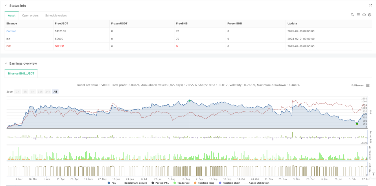
start: 2024-02-21 00:00:00
end: 2025-02-18 08:00:00
period: 1h
basePeriod: 1h
exchanges: [{"eid":"Binance","currency":"BNB_USDT"}]
*/

//@version=6
strategy("Multi-Band Comparison Strategy with Separate Entry/Exit Confirmation", overlay=true, 
         default_qty_type=strategy.percent_of_equity, default_qty_value=10, 
         initial_capital=5000, currency=currency.USD)

// === Inputs ===

// Basic Parameters
length         = input.int(20, "Length (SMA)", minval=1)
boll_mult      = input.float(1.0, "Bollinger Band Multiplier", minval=0.1, step=0.1)
upper_quantile = input.float(0.95, "Upper Quantile (0.0-1.0)", minval=0.0, maxval=1.0)
lower_quantile = input.float(0.05, "Lower Quantile (0.0-1.0)", minval=0.0, maxval=1.0)

// Separate confirmation inputs
entry_confirmBars = input.int(1, "Entry Confirmation Bars", minval=1, tooltip="Number of consecutive bars the entry condition must hold")
exit_confirmBars  = input.int(1, "Exit Confirmation Bars",  minval=1, tooltip="Number of consecutive bars the exit condition must hold")

// Toggle Visibility for Bands
show_lower_boll  = input.bool(false, "Show Lower Bollinger Band", tooltip="Enable or disable the lower Bollinger Band")
show_upper_boll  = input.bool(true,  "Show Upper Bollinger Band", tooltip="Enable or disable the upper Bollinger Band")
show_lower_quant = input.bool(true, "Show Lower Quantile Band", tooltip="Enable or disable the lower Quantile Band")
show_upper_quant = input.bool(true,  "Show Upper Quantile Band", tooltip="Enable or disable the upper Quantile Band")
show_upper_power = input.bool(true,  "Show Upper Power-Law Band", tooltip="Enable or disable the upper Power-Law Band")
show_lower_power = input.bool(false, "Show Lower Power-Law Band", tooltip="Enable or disable the lower Power-Law Band")
show_quant_std   = input.bool(true,  "Show Standard Deviation around Quantile Bands", tooltip="Enable or disable standard deviation lines around Quantile Bands")

// Individual Toggles for Std Dev Lines
show_upper_quant_std_up   = input.bool(true,  "Show Upper Quantile + Std Dev", tooltip="Enable or disable the Upper Quantile + Std Dev line")
show_upper_quant_std_down = input.bool(true,  "Show Upper Quantile - Std Dev", tooltip="Enable or disable the Upper Quantile - Std Dev line")
show_lower_quant_std_up   = input.bool(false, "Show Lower Quantile + Std Dev", tooltip="Enable or disable the Lower Quantile + Std Dev line")
show_lower_quant_std_down = input.bool(true,  "Show Lower Quantile - Std Dev", tooltip="Enable or disable the Lower Quantile - Std Dev line")

// Moving Average Toggles
show_ema = input.bool(false, "Show EMA", tooltip="Enable or disable the Exponential Moving Average")
show_sma = input.bool(false, "Show SMA", tooltip="Enable or disable the Simple Moving Average")

// EMA Parameters
ema_length = input.int(50, minval=1, title="EMA Length")
ema_source = input.source(close, title="EMA Source")

// === Data Handling ===

// Create persistent arrays to store data
var float[] data_array   = array.new_float()
var float[] return_array = array.new_float()

// Update the data array with the latest close prices
if array.size(data_array) < length
    array.push(data_array, close)
else
    array.shift(data_array)
    array.push(data_array, close)

// Update the return array with the latest returns
returns = close / close[1] - 1
if array.size(return_array) < length
    array.push(return_array, returns)
else
    array.shift(return_array)
    array.push(return_array, returns)

// === Helper Function ===

// Function to calculate a custom percentile
f_percentile(arr, quantile) =>
    arr_sorted = array.copy(arr)
    array.sort(arr_sorted, order.ascending)
    index = math.round((array.size(arr_sorted) - 1) * quantile)
    array.get(arr_sorted, index)

// === Calculations ===

// Bollinger Bands Calculation
sma        = ta.sma(close, length)
stdev      = ta.stdev(close, length)
boll_upper = sma + boll_mult * stdev
boll_lower = sma - boll_mult * stdev

// Power-Law Bands Calculation
var float power_upper = na
var float power_lower = na
if array.size(return_array) == length
    power_upper := f_percentile(return_array, upper_quantile)
    power_lower := f_percentile(return_array, lower_quantile)
var float power_upper_band = na
var float power_lower_band = na
if not na(power_upper) and not na(power_lower)
    power_upper_band := close * (1 + power_upper)
    power_lower_band := close * (1 + power_lower)

// Quantile Bands Calculation
var float quant_upper = na
var float quant_lower = na
if array.size(data_array) == length
    quant_upper := f_percentile(data_array, upper_quantile)
    quant_lower := f_percentile(data_array, lower_quantile)

// Standard Deviation around Quantile Bands
quant_upper_std_up   = quant_upper + stdev
quant_upper_std_down = quant_upper - stdev
quant_lower_std_up   = quant_lower + stdev
quant_lower_std_down = quant_lower - stdev

// === Color Calculations ===

// For the upper Bollinger band, color it yellow when price is above it, black otherwise.
upper_boll_color = close > boll_upper ? color.yellow : color.black

// The entry/exit trigger is based on the lower std dev band of the upper quantile band.
// It "turns green" (i.e. favorable for entry) when the price is above this level,
// and "turns red" (i.e. unfavorable, triggering an exit) when price is below it.
triggerCondition = close > quant_upper_std_down

// For plotting purposes, define the color of the lower std dev band of the upper quantile band:
triggerColor = triggerCondition ? color.green : color.red

// (Other color definitions remain for the additional bands.)
upper_power_color = (not na(power_upper_band) and not na(quant_upper_std_up) and power_upper_band > quant_upper_std_up) ? color.new(#FF00FF, 0) : color.black
upper_quant_color = (not na(quant_upper) and not na(power_upper_band) and power_upper_band > quant_upper) ? color.new(#FFAE00, 0) : color.rgb(50, 50, 50)
upper_quant_std_down_color = (not na(quant_upper_std_down) and close > quant_upper_std_down) ? color.green : color.red
lower_quant_std_down_color = (not na(quant_lower_std_down) and close > quant_lower_std_down) ? color.rgb(24, 113, 0, 44) : color.red
lower_quant_color = (ta.cross(close, quant_lower) or close == quant_lower) ? color.red : color.rgb(0, 238, 255)

// For demonstration, a variable to toggle a color on the Bollinger crossover.
var color upper_quant_std_up_color = color.black
if ta.crossover(close, boll_upper)
    upper_quant_std_up_color := color.yellow
if ta.crossunder(close, boll_upper)
    upper_quant_std_up_color := color.black

// === Confirmation Bars Logic with Separate Counters Based on Trigger Condition ===

// Use the trigger condition (based on the lower std dev band of the upper quantile band)
// for entry/exit confirmation.
var int entryCounter = 0
var int exitCounter  = 0

// When triggerCondition is true (price above quant_upper_std_down) the "green" state holds.
entryCounter := triggerCondition ? entryCounter + 1 : 0
// When triggerCondition is false (price below quant_upper_std_down) the "red" state holds.
exitCounter  := not triggerCondition ? exitCounter + 1 : 0

// === Strategy Orders ===

// Enter long when triggerCondition has been true for at least entry_confirmBars bars and no position is active.
if (entryCounter >= entry_confirmBars) and (strategy.position_size <= 0)
    strategy.entry("Long", strategy.long)

// Exit long when triggerCondition has been false for at least exit_confirmBars bars and a long position is active.
if (exitCounter >= exit_confirmBars) and (strategy.position_size > 0)
    strategy.close("Long")

// === Plotting ===

// Plot Bollinger Bands
plot(show_upper_boll ? boll_upper : na, color=upper_boll_color, title="Bollinger Upper", linewidth=2)
plot(show_lower_boll ? boll_lower : na, color=color.red, title="Bollinger Lower", linewidth=1)

// Plot Power-Law Bands
plot(show_upper_power ? power_upper_band : na, color=upper_power_color, title="Power-Law Upper", linewidth=1)
plot(show_lower_power ? power_lower_band : na, color=color.rgb(255, 59, 248), title="Power-Law Lower", linewidth=1)

// Plot Quantile Bands
plot(show_upper_quant ? quant_upper : na, color=upper_quant_color, title="Quantile Upper", linewidth=1)
plot(show_lower_quant ? quant_lower : na, color=lower_quant_color, title="Quantile Lower", linewidth=1)

// Plot Standard Deviation around Quantile Bands
plot(show_quant_std and show_upper_quant and show_upper_quant_std_up ? quant_upper_std_up : na, color=upper_quant_std_up_color, title="Quantile Upper + Std Dev", linewidth=2)
plot(show_quant_std and show_upper_quant and show_upper_quant_std_down ? quant_upper_std_down : na, color=upper_quant_std_down_color, title="Quantile Upper - Std Dev", linewidth=2)
plot(show_quant_std and show_lower_quant and show_lower_quant_std_up ? quant_lower_std_up : na, color=color.green, title="Quantile Lower + Std Dev", linewidth=1)
plot(show_quant_std and show_lower_quant and show_lower_quant_std_down ? quant_lower_std_down : na, color=lower_quant_std_down_color, title="Quantile Lower - Std Dev", linewidth=1)

// Also plot the trigger line (lower std dev band of upper quantile band) with its own color
plot(show_quant_std ? quant_upper_std_down : na, color=triggerColor, title="Trigger (Lower Std Dev of Upper Quantile)", linewidth=2)

// Plot SMA for reference
plot(show_sma ? sma : na, color=color.rgb(0, 24, 132), title="SMA", linewidth=3)

// Plot EMA for reference
ema_value = ta.ema(ema_source, ema_length)
plot(show_ema ? ema_value : na, color=color.rgb(147, 0, 0), title="EMA", linewidth=2)