
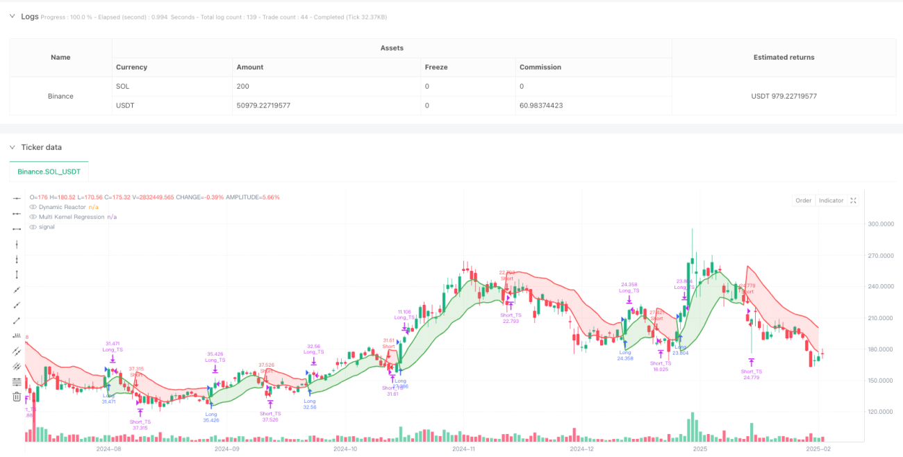
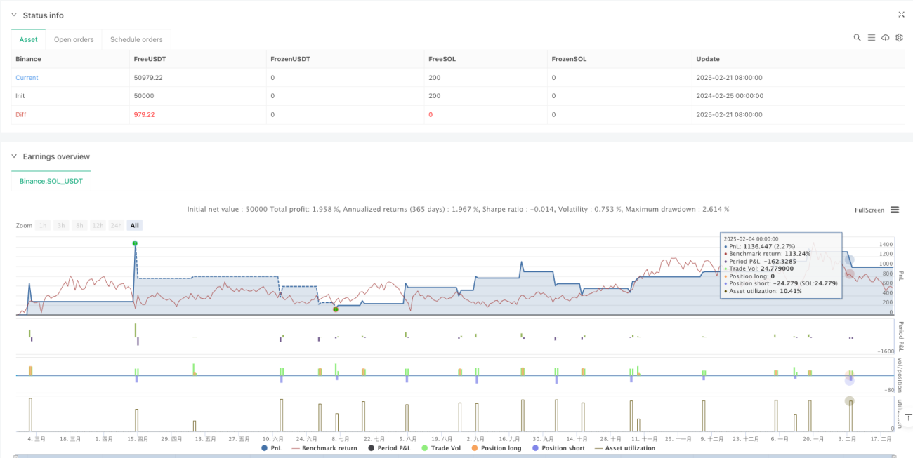
Descripción general
La estrategia es un sistema de seguimiento de tendencias que combina Dynamic Reactor y Multi-Kernel Regression. Captura las tendencias del mercado mediante la combinación de la vía ATR, la media SMA y la regresión de Gauss con la regresión de Epanechnikov, y utiliza el indicador RSI para filtrar las señales. La estrategia también incluye un sistema completo de gestión de posiciones, que incluye funciones como stop loss dinámico, objetivos de multiplicación de ganancias y seguimiento de stop loss.
Principio de estrategia
El núcleo de la estrategia se compone de dos partes principales: la primera es el reactor dinámico (DR), que construye un canal de precios adaptado basado en el ATR y el SMA. El ancho del canal está determinado por el multiplicador ATR y la posición del canal se ajusta con el movimiento del SMA.
Ventajas estratégicas
- Adaptabilidad: mediante la combinación de reactores dinámicos y regresión multicore, la estrategia puede adaptarse automáticamente a diferentes entornos y condiciones de fluctuación del mercado.
- La gestión de riesgos es perfecta: incluye múltiples mecanismos de control de riesgos, como el deterioro dinámico, el reparto de ganancias y el seguimiento del deterioro.
- Alta calidad de la señal: Con el filtro RSI y la confirmación cruzada de las dos líneas, se puede reducir efectivamente la señal falsa.
- Alta eficiencia de cálculo: Aunque se utiliza un complejo algoritmo de regresión nuclear, se garantiza el rendimiento en tiempo real de las estrategias mediante la optimización de los métodos de cálculo.
Riesgo estratégico
- Sensibilidad de parámetros: la eficacia de la estrategia depende en gran medida de la configuración de parámetros como el multiplicador de ATR y el ancho de banda de la función nuclear. Los parámetros inadecuados pueden causar exceso de comercio o oportunidades perdidas.
- Retraso: debido al uso de promedios móviles y algoritmos de regresión, puede haber un cierto retraso en el movimiento rápido.
- Adaptabilidad al mercado: la estrategia funciona mejor en mercados de tendencia, pero puede generar falsas señales con frecuencia en mercados de oscilación intermedia.
- Complejidad de cálculo: El cálculo de la parte de regresión de múltiples núcleos es más complejo y se debe prestar atención a la optimización de rendimiento en el entorno de transacciones de alta frecuencia.
Dirección de optimización de la estrategia
- Adaptación de parámetros: Se puede introducir un mecanismo de adaptación para ajustar dinámicamente el multiplicador ATR y el ancho de banda de la función nuclear según las fluctuaciones del mercado.
- Optimización de la señal: Considere agregar indicadores auxiliares como volumen de ventas, configuración de precios, etc., para mejorar la fiabilidad de la señal.
- Control de riesgos: la proporción de objetivos de stop loss y profit puede ajustarse a la fluctuación del mercado.
- Filtrado de mercado: agregar módulos de identificación de entornos de mercado para usar diferentes estrategias de negociación en diferentes condiciones de mercado.
Resumir
Se trata de un sistema de negociación completo que combina métodos estadísticos modernos y análisis técnico tradicional. A través de una combinación innovadora de reactores dinámicos y regresión multi-núcleo, así como un mecanismo de gestión de riesgos perfectos, la estrategia muestra una buena adaptabilidad y estabilidad. Si bien hay algunos lugares que necesitan ser optimizados, la estrategia espera mantener un rendimiento estable en diferentes entornos de mercado a través de la mejora continua y la optimización de parámetros.
/*backtest
start: 2024-07-20 00:00:00
end: 2025-07-19 08:00:00
period: 1d
basePeriod: 1d
exchanges: [{"eid":"Binance","currency":"ETH_USDT","balance":2000000}]
*/

//@version=5
strategy("DR+MKR Signals – Band SL, Multiple TP & Trailing Stop", overlay=true, default_qty_value=10)

// =====================================================================- 1