Aperçu

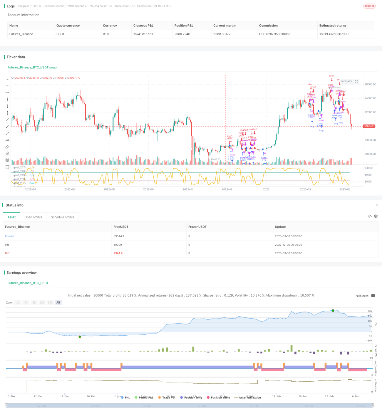
Cette stratégie utilise l'indicateur de force relative (RSI) ou l'indicateur de flux de trésorerie (MFI) pour déterminer si le marché est haussier ou baissier et, combiné au coefficient de hausse et de baisse de la théorie Dow, pour calculer la distribution de probabilité ajustée. Selon les différents types de marché, différentes logiques d'entrée et de sortie sont utilisées.

Principe de stratégie

1. Calculer le RSI ou MFI pour déterminer l'état actuel du marché (bull ou bear)
2. Coefficient de Dow pour calculer le coefficient de Bull et de Bear, qui reflète la corrélation entre les prix actuels et le volume des transactions
3. Ajuster la distribution de probabilité RSI/MFI pour déterminer une distribution plus large avec précision
4. Déterminer si une session est acceptée en fonction de l'identifiant de session et de la probabilité
5. Stop loss lorsque les bénéfices sont retirés ou que le marché se calme

Analyse des avantages

1. La théorie de la dynamique, combinée à la théorie de la dynamique, permet d'évaluer plus précisément le type de marché.
2. Éviter l'admission à l'aveugle en tenant compte des facteurs d'ajustement
3. Haute marge bénéficiaire, bas retrait

Analyse des risques

1. Les paramètres ne sont pas à la bonne heure, cela peut entraîner de nombreuses erreurs de jugement
2. Il faut un soutien historique suffisant.
3. La logique d'arrêt des pertes est simple et ne peut pas être optimisée pour des situations spécifiques.

Direction d'optimisation

1. Il est possible de considérer d'autres indicateurs pour juger de la session de marché.
2. Ajout de logiques de stop-loss plus rigoureuses basées sur la volatilité et les données historiques
3. Vous pouvez essayer d'identifier de meilleurs paramètres avec l'apprentissage automatique.

Résumer

Cette stratégie est généralement bien testée et a une certaine valeur de combat. Cependant, des tests et des ajustements supplémentaires sont nécessaires, en particulier la logique d'arrêt des pertes. L'utilisation d'indicateurs d'aide au jugement est plus efficace et ne peut pas être suivie à l'aveugle.