Stratégie de trading Bitcoin basée sur des indicateurs quantitatifs
Aperçu
Cette stratégie utilise plusieurs indicateurs quantitatifs pour déterminer le moment d’achat et de vente de Bitcoin, permettant des transactions automatisées. Il s’agit principalement de l’indicateur Hull, de l’indicateur de force relative (RSI), des bandes de Brin (BB) et de l’oscillateur de volume de transaction (VO).
Principe de stratégie
L’utilisation d’une moyenne mobile de Hull modifiée pour déterminer la direction de la tendance principale du marché, combinée à une aide de la ceinture de Brin pour déterminer les points de rupture.
L’indicateur RSI émet un signal de transaction en combinant une zone de survente et de survente pour juger de la zone de survente et de survente adaptée à la zone de fluctuation. Il définit également deux ensembles de paramètres pour vérifier le signal de duplicate.
L’oscillateur de transaction détermine la direction des ventes et des achats, et évite les fausses ruptures.
La gestion des risques est assurée en prévoyant un stop loss en fonction du ratio stop loss/stop loss.
Analyse des avantages
La courbe de Hull permet de capturer plus rapidement les changements de tendance, et le jugement auxiliaire de Brin permet de réduire les faux signaux.
Les paramètres de l’indicateur RSI sont optimisés et la vérification des signaux en double est plus fiable.
L’oscillateur de volume de transaction combine les signaux de tendance et d’indicateur pour éviter les transactions inexactes.
La méthode d’arrêt de perte prédéfinie permet de contrôler automatiquement les pertes individuelles et de contrôler efficacement les risques globaux.
Analyse des risques
Une mauvaise configuration des paramètres peut entraîner une fréquence de transaction trop élevée ou une mauvaise efficacité du signal.
Si un événement soudain entraîne une forte volatilité du marché, le stop-loss peut être franchi et entraîner une perte importante.
Les paramètres doivent être re-testés et optimisés lors de l’échange d’une variété d’échange contre une autre.
L’oscillateur de transaction est désactivé lorsque les données de transaction sont manquantes.
Direction d’optimisation
Les paramètres RSI sont testés en combinaison pour trouver le paramètre optimal.
Essayez d’utiliser d’autres indicateurs comme le MACD, le KD, etc. en combinaison avec le RSI pour améliorer la précision du signal.
Ajout d’un module de prévision de modèle, combiné à l’apprentissage automatique, pour déterminer la direction du marché.
Test de l’effet des paramètres sur d’autres variétés commerciales.
Optimiser les algorithmes de stop-loss pour maximiser les bénéfices
Résumer
Cette stratégie utilise un ensemble d’indicateurs techniques quantitatifs pour déterminer le moment de l’achat et de la vente. La négociation automatisée de Bitcoin est réalisée par des méthodes telles que l’optimisation des paramètres et le contrôle des risques. L’efficacité est bonne, mais il faut continuer à tester et à optimiser pour s’adapter aux changements du marché.
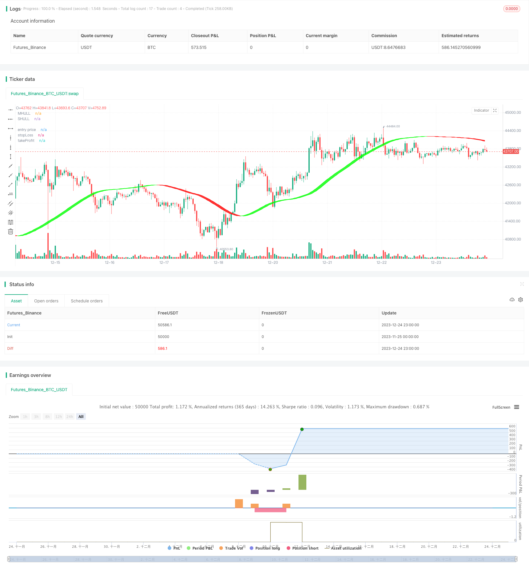
/*backtest
start: 2023-11-25 00:00:00
end: 2023-12-25 00:00:00
period: 1h
basePeriod: 15m
exchanges: [{"eid":"Futures_Binance","currency":"BTC_USDT"}]
*/


// © maxencetajet

//@version=5
strategy("Strategy Crypto", overlay=true, initial_capital=1000, default_qty_type=strategy.fixed, default_qty_value=0.5, slippage=25)

src1 = input.source(close, title="Source")
target_stop_ratio = input.float(title='Risk/Reward', defval=1.5, minval=0.5, maxval=100)

startDate = input.int(title='Start Date', defval=1, minval=1, maxval=31, group="beginning Backtest")
startMonth = input.int(title='Start Month', defval=5, minval=1, maxval=12, group="beginning Backtest")
startYear = input.int(title='Start Year', defval=2022, minval=2000, maxval=2100, group="beginning Backtest")

inDateRange = time >= timestamp(syminfo.timezone, startYear, startMonth, startDate, 0, 0)

swingHighV = input.int(7, title="Swing High", group="number of past candles")
swingLowV = input.int(7, title="Swing Low", group="number of past candles")

//Hull Suite

modeSwitch = input.string("Hma", title="Hull Variation", options=["Hma", "Thma", "Ehma"], group="Hull Suite")
length = input(60, title="Length", group="Hull Suite")
lengthMult = input(3, title="Length multiplier", group="Hull Suite")

HMA(_src1, _length) =>
    ta.wma(2 * ta.wma(_src1, _length / 2) - ta.wma(_src1, _length), math.round(math.sqrt(_length)))

EHMA(_src1, _length) =>
    ta.ema(2 * ta.ema(_src1, _length / 2) - ta.ema(_src1, _length), math.round(math.sqrt(_length)))

THMA(_src1, _length) =>
    ta.wma(ta.wma(_src1, _length / 3) * 3 - ta.wma(_src1, _length / 2) - ta.wma(_src1, _length), _length)

Mode(modeSwitch, src1, len) =>
    modeSwitch == 'Hma' ? HMA(src1, len) : modeSwitch == 'Ehma' ? EHMA(src1, len) : modeSwitch == 'Thma' ? THMA(src1, len / 2) : na

_hull = Mode(modeSwitch, src1, int(length * lengthMult))
HULL = _hull
MHULL = HULL[0]
SHULL = HULL[2]

hullColor = HULL > HULL[2] ? #00ff00 : #ff0000

Fi1 = plot(MHULL, title='MHULL', color=hullColor, linewidth=1, transp=50)
Fi2 = plot(SHULL, title='SHULL', color=hullColor, linewidth=1, transp=50)
fill(Fi1, Fi2, title='Band Filler', color=hullColor, transp=40)

//QQE MOD

RSI_Period = input(6, title='RSI Length', group="QQE MOD")
SF = input(5, title='RSI Smoothing', group="QQE MOD")
QQE = input(3, title='Fast QQE Factor', group="QQE MOD")
ThreshHold = input(3, title='Thresh-hold', group="QQE MOD")

src = input(close, title='RSI Source', group="QQE MOD")

Wilders_Period = RSI_Period * 2 - 1

Rsi = ta.rsi(src, RSI_Period)
RsiMa = ta.ema(Rsi, SF)
AtrRsi = math.abs(RsiMa[1] - RsiMa)
MaAtrRsi = ta.ema(AtrRsi, Wilders_Period)
dar = ta.ema(MaAtrRsi, Wilders_Period) * QQE

longband = 0.0
shortband = 0.0
trend = 0

DeltaFastAtrRsi = dar
RSIndex = RsiMa
newshortband = RSIndex + DeltaFastAtrRsi
newlongband = RSIndex - DeltaFastAtrRsi
longband := RSIndex[1] > longband[1] and RSIndex > longband[1] ? math.max(longband[1], newlongband) : newlongband
shortband := RSIndex[1] < shortband[1] and RSIndex < shortband[1] ? math.min(shortband[1], newshortband) : newshortband
cross_1 = ta.cross(longband[1], RSIndex)
trend := ta.cross(RSIndex, shortband[1]) ? 1 : cross_1 ? -1 : nz(trend[1], 1)
FastAtrRsiTL = trend == 1 ? longband : shortband

length1 = input.int(50, minval=1, title='Bollinger Length', group="QQE MOD")
mult = input.float(0.35, minval=0.001, maxval=5, step=0.1, title='BB Multiplier', group="QQE MOD")
basis = ta.sma(FastAtrRsiTL - 50, length1)
dev = mult * ta.stdev(FastAtrRsiTL - 50, length1)
upper = basis + dev
lower = basis - dev
color_bar = RsiMa - 50 > upper ? #00c3ff : RsiMa - 50 < lower ? #ff0062 : color.gray

QQEzlong = 0
QQEzlong := nz(QQEzlong[1])
QQEzshort = 0
QQEzshort := nz(QQEzshort[1])
QQEzlong := RSIndex >= 50 ? QQEzlong + 1 : 0
QQEzshort := RSIndex < 50 ? QQEzshort + 1 : 0

RSI_Period2 = input(6, title='RSI Length', group="QQE MOD")
SF2 = input(5, title='RSI Smoothing', group="QQE MOD")
QQE2 = input(1.61, title='Fast QQE2 Factor', group="QQE MOD")
ThreshHold2 = input(3, title='Thresh-hold', group="QQE MOD")

src2 = input(close, title='RSI Source', group="QQE MOD")

Wilders_Period2 = RSI_Period2 * 2 - 1

Rsi2 = ta.rsi(src2, RSI_Period2)
RsiMa2 = ta.ema(Rsi2, SF2)
AtrRsi2 = math.abs(RsiMa2[1] - RsiMa2)
MaAtrRsi2 = ta.ema(AtrRsi2, Wilders_Period2)
dar2 = ta.ema(MaAtrRsi2, Wilders_Period2) * QQE2
longband2 = 0.0
shortband2 = 0.0
trend2 = 0

DeltaFastAtrRsi2 = dar2
RSIndex2 = RsiMa2
newshortband2 = RSIndex2 + DeltaFastAtrRsi2
newlongband2 = RSIndex2 - DeltaFastAtrRsi2
longband2 := RSIndex2[1] > longband2[1] and RSIndex2 > longband2[1] ? math.max(longband2[1], newlongband2) : newlongband2
shortband2 := RSIndex2[1] < shortband2[1] and RSIndex2 < shortband2[1] ? math.min(shortband2[1], newshortband2) : newshortband2
cross_2 = ta.cross(longband2[1], RSIndex2)
trend2 := ta.cross(RSIndex2, shortband2[1]) ? 1 : cross_2 ? -1 : nz(trend2[1], 1)
FastAtrRsi2TL = trend2 == 1 ? longband2 : shortband2

QQE2zlong = 0
QQE2zlong := nz(QQE2zlong[1])
QQE2zshort = 0
QQE2zshort := nz(QQE2zshort[1])
QQE2zlong := RSIndex2 >= 50 ? QQE2zlong + 1 : 0
QQE2zshort := RSIndex2 < 50 ? QQE2zshort + 1 : 0

hcolor2 = RsiMa2 - 50 > ThreshHold2 ? color.silver : RsiMa2 - 50 < 0 - ThreshHold2 ? color.silver : na

Greenbar1 = RsiMa2 - 50 > ThreshHold2
Greenbar2 = RsiMa - 50 > upper

Redbar1 = RsiMa2 - 50 < 0 - ThreshHold2
Redbar2 = RsiMa - 50 < lower

//Volume Oscillator

var cumVol = 0.
cumVol += nz(volume)
if barstate.islast and cumVol == 0
    runtime.error("No volume is provided by the data vendor.")
shortlen = input.int(5, minval=1, title = "Short Length", group="Volume Oscillator")
longlen = input.int(10, minval=1, title = "Long Length", group="Volume Oscillator")
short = ta.ema(volume, shortlen)
long = ta.ema(volume, longlen)
osc = 100 * (short - long) / long

//strategy

enterLong   =  '    {  "message_type": "bot",  "bot_id": 4635591,  "email_token": "25byourtefcodeuufyd2-43314-ab98-bjorg224",  "delay_seconds": 1}  ' //start long deal

ExitLong    =  '    {  "message_type": "bot",  "bot_id": 4635591,  "email_token": "25byourtefcodeuufyd2-43314-ab98-bjorg224",  "delay_seconds": 0,  "action": "close_at_market_price"}  ' // close long deal market

enterShort  =  '    {  "message_type": "bot",  "bot_id": 4635690,  "email_token": "25byourtefcodeuufyd2-43314-ab98-bjorg224",  "delay_seconds": 1}  ' // start short deal

ExitShort   =  '    {  "message_type": "bot",  "bot_id": 4635690,  "email_token": "25byourtefcodeuufyd2-43314-ab98-bjorg224",  "delay_seconds": 0,  "action": "close_at_market_price"}  ' // close short deal market

longcondition = close > MHULL and HULL > HULL[2] and osc > 0 and Greenbar1 and Greenbar2 and not Greenbar1[1] and not Greenbar2[1]
shortcondition = close < SHULL and HULL < HULL[2] and osc > 0 and Redbar1 and Redbar2 and not Redbar1[1] and not Redbar2[1]

float risk_long = na
float risk_short = na
float stopLoss = na
float takeProfit = na
float entry_price = na

risk_long := risk_long[1]
risk_short := risk_short[1]

swingHigh = ta.highest(high, swingHighV)
swingLow = ta.lowest(low, swingLowV)

if strategy.position_size == 0 and longcondition and inDateRange
    risk_long := (close - swingLow) / close
    strategy.entry("long", strategy.long, comment="Buy", alert_message=enterLong)

if strategy.position_size == 0 and shortcondition and inDateRange
    risk_short := (swingHigh - close) / close
    strategy.entry("short", strategy.short, comment="Sell", alert_message=enterShort)

if strategy.position_size > 0

    stopLoss := strategy.position_avg_price * (1 - risk_long)
    takeProfit := strategy.position_avg_price * (1 + target_stop_ratio * risk_long)
    entry_price := strategy.position_avg_price
    strategy.exit("long exit", "long", stop = stopLoss, limit = takeProfit, alert_message=ExitLong)

if strategy.position_size < 0

    stopLoss := strategy.position_avg_price * (1 + risk_short)
    takeProfit := strategy.position_avg_price * (1 - target_stop_ratio * risk_short)
    entry_price := strategy.position_avg_price
    strategy.exit("short exit", "short", stop = stopLoss, limit = takeProfit, alert_message=ExitShort)

p_ep = plot(entry_price, color=color.new(color.white, 0), linewidth=2, style=plot.style_linebr, title='entry price')
p_sl = plot(stopLoss, color=color.new(color.red, 0), linewidth=2, style=plot.style_linebr, title='stopLoss')
p_tp = plot(takeProfit, color=color.new(color.green, 0), linewidth=2, style=plot.style_linebr, title='takeProfit')
fill(p_sl, p_ep, color.new(color.red, transp=85))
fill(p_tp, p_ep, color.new(color.green, transp=85))