Stratégie de trading quantitative de divergence CVD
Une vue d’ensemble de la stratégie: La stratégie utilise les indicateurs de CVD et les écarts de formation de prix pour capturer les signaux potentiels de revers de tendance. La stratégie calcule les indicateurs de CVD et, en les comparant aux prix, détermine s’il s’agit d’un écarts de hausse ou de baisse.
Le principe de la stratégie:
- Calculer l’indicateur de CVD: calculer l’indicateur de CVD et sa moyenne mobile en fonction du volume d’affaires et du volume d’affaires à vide.
- Identifier les déviations: déterminer si des déviations se sont formées en comparant les hauts et les bas de l’indicateur CVD avec les hauts et les bas du prix.
- Le prix de l’innovation est faible, mais l’indicateur CVD se forme à des niveaux plus élevés
- Les prix sont à la hausse, mais les indices de CVD sont plus bas
- Déviation de la baisse habituelle: les prix sont à nouveau élevés, mais l’indicateur CVD forme des sommets plus bas
- L’indicateur CVD forme des sommets plus élevés
- Ouverture de position: lorsque le signal de déviation est détecté, ouverture de position en plus ou en moins selon le type de déviation.
- Stop loss: utilisation d’un stop mobile et d’un stop à pourcentage fixe. Le prix stop est calculé en fonction du prix d’ouverture multiplié par le pourcentage stop loss. Le prix stop est calculé en fonction du prix d’ouverture multiplié par le pourcentage stop loss.
- Le placement de la pyramide: la stratégie permet un placement de la pyramide avec un maximum de 3 positions.
Avantages stratégiques:
- Signal de renversement de tendance: L’écart de CVD est un signal de renversement de tendance efficace qui peut aider à saisir les occasions de renversement de tendance.
- Signaux de continuation de la tendance: les déviations cachées peuvent servir de signaux de continuation de la tendance et aider la stratégie à rester dans la bonne direction dans la tendance.
- Contrôle du risque: Le risque est contrôlé efficacement avec des stop-loss mobiles et des stop-loss à pourcentage fixe.
- La pyramide de mise en position: permet de mettre en place de nombreuses positions afin de mieux exploiter les tendances.
Les risques stratégiques:
- La validité du signal: le signal déviant n’est pas entièrement fiable, il peut parfois y avoir des faux signaux.
- Configuration des paramètres: les résultats de la stratégie sont sensibles à la configuration des paramètres, et différents paramètres peuvent entraîner des résultats différents.
- Le point de glissement de stop-loss: dans des conditions extrêmes, un stop-loss peut ne pas être négocié au prix par défaut, ce qui entraîne un risque supplémentaire.
- Frais de transaction: la fréquence des positions ouvertes peut entraîner des frais de transaction plus élevés, affectant les gains stratégiques.
Les directions d’optimisation
- Optimisation des paramètres dynamiques: paramètres qui s’adaptent aux différentes conditions du marché et améliorent l’efficacité du signal.
- Combinaison avec d’autres indicateurs: Combinaison avec d’autres indicateurs techniques tels que le RSI, le MACD, etc., pour améliorer la fiabilité du signal.
- Amélioration de l’arrêt de perte: adopter des stratégies d’arrêt de perte plus avancées, telles que le suivi des arrêts, l’arrêt de la volatilité, etc.
- Gestion de la taille des positions: Adaptez la taille des positions en fonction des fluctuations du marché, des fonds du compte, etc.
Résumé: La stratégie de trading CVD déviant de la quantité permet de capturer le déviement de l’indicateur CVD par rapport au prix et d’identifier les opportunités potentielles de renversement de tendance. Elle utilise également des stop-loss mobiles et des stop-loss à pourcentage fixe pour contrôler le risque. Le principal avantage de la stratégie réside dans la capacité de capturer efficacement les signaux de renversement de tendance et de prolongation, et de mieux maîtriser la tendance grâce à la prise de position de la pyramide.
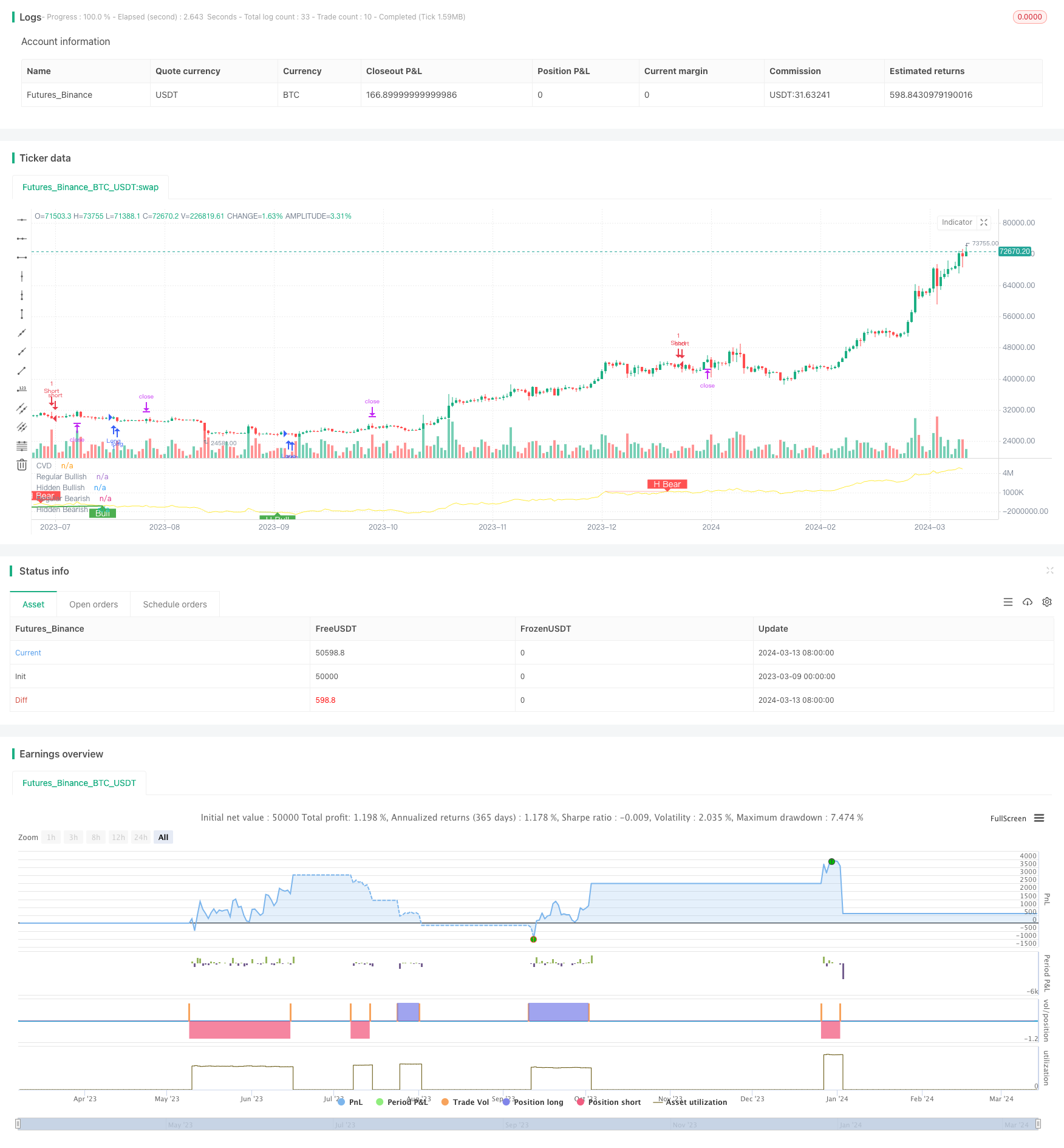
/*backtest
start: 2023-03-09 00:00:00
end: 2024-03-14 00:00:00
period: 1d
basePeriod: 1h
exchanges: [{"eid":"Futures_Binance","currency":"BTC_USDT"}]
*/

// This source code is subject to the terms of the Mozilla Public License 2.0 at https://mozilla.org/MPL/2.0/

//@version=5
//@ mmattman

//Thank you to @ contrerae and Tradingview each for parts of the code to make
//this indicator and matching strategy and also theCrypster for the clean concise TP/SL code.

// indicator(title="CVD Divergence Indicator 1", shorttitle='CVD Div1', format=format.price, timeframe="", timeframe_gaps=true)

strategy("CVD Divergence Strategy.1.mm", shorttitle = 'CVD Div Str 1', overlay=false)


//..................................................................................................................
// Inputs
periodMa = input.int(title='MA Length', minval=1, defval=20)
plotMa = input(title='Plot MA?', defval=false)

// Calculations (Bull & Bear Balance Indicator by Vadim Gimelfarb)
iff_1 = close[1] < open ? math.max(high - close[1], close - low) : math.max(high - open, close - low)
iff_2 = close[1] > open ? high - low : math.max(open - close[1], high - low)
iff_3 = close[1] < open ? math.max(high - close[1], close - low) : high - open
iff_4 = close[1] > open ? high - low : math.max(open - close[1], high - low)
iff_5 = close[1] < open ? math.max(open - close[1], high - low) : high - low
iff_6 = close[1] > open ? math.max(high - open, close - low) : iff_5
iff_7 = high - close < close - low ? iff_4 : iff_6
iff_8 = high - close > close - low ? iff_3 : iff_7
iff_9 = close > open ? iff_2 : iff_8
bullPower = close < open ? iff_1 : iff_9
iff_10 = close[1] > open ? math.max(close[1] - open, high - low) : high - low
iff_11 = close[1] > open ? math.max(close[1] - low, high - close) : math.max(open - low, high - close)
iff_12 = close[1] > open ? math.max(close[1] - open, high - low) : high - low
iff_13 = close[1] > open ? math.max(close[1] - low, high - close) : open - low
iff_14 = close[1] < open ? math.max(open - low, high - close) : high - low
iff_15 = close[1] > open ? math.max(close[1] - open, high - low) : iff_14
iff_16 = high - close < close - low ? iff_13 : iff_15
iff_17 = high - close > close - low ? iff_12 : iff_16
iff_18 = close > open ? iff_11 : iff_17
bearPower = close < open ? iff_10 : iff_18

// Calculations (Bull & Bear Pressure Volume)
bullVolume = bullPower / (bullPower + bearPower) * volume
bearVolume = bearPower / (bullPower + bearPower) * volume

// Calculations Delta
delta = bullVolume - bearVolume
cvd = ta.cum(delta)
cvdMa = ta.sma(cvd, periodMa)

// Plotting
customColor = cvd > cvdMa ? color.new(color.teal, 50) : color.new(color.red, 50)
plotRef1 = plot(cvd, style=plot.style_line, linewidth=1, color=color.new(color.yellow, 0), title='CVD')
plotRef2 = plot(plotMa ? cvdMa : na, style=plot.style_line, linewidth=1, color=color.new(color.white, 0), title='CVD MA')
fill(plotRef1, plotRef2, color=customColor)
//..................................................................................................................


// len = input.int(title="RSI Period", minval=1, defval=14)
// src = input(title="RSI Source", defval=close)
lbR = input(title="Pivot Lookback Right", defval=3)
lbL = input(title="Pivot Lookback Left", defval=7)
rangeUpper = input(title="Max of Lookback Range", defval=60)
rangeLower = input(title="Min of Lookback Range", defval=5)
plotBull = input(title="Plot Bullish", defval=true)
plotHiddenBull = input(title="Plot Hidden Bullish", defval=true)
plotBear = input(title="Plot Bearish", defval=true)
plotHiddenBear = input(title="Plot Hidden Bearish", defval=true)
bearColor = color.red
bullColor = color.green
hiddenBullColor = color.new(color.green, 80)
hiddenBearColor = color.new(color.red, 80)
textColor = color.white
noneColor = color.new(color.white, 100)
osc = cvd

// plot(osc, title="CVD", linewidth=2, color=#2962FF)
// hline(50, title="Middle Line", color=#787B86, linestyle=hline.style_dotted)
// obLevel = hline(70, title="Overbought", color=#787B86, linestyle=hline.style_dotted)
// osLevel = hline(30, title="Oversold", color=#787B86, linestyle=hline.style_dotted)
// fill(obLevel, osLevel, title="Background", color=color.rgb(33, 150, 243, 90))

plFound = na(ta.pivotlow(osc, lbL, lbR)) ? false : true
phFound = na(ta.pivothigh(osc, lbL, lbR)) ? false : true
_inRange(cond) =>
	bars = ta.barssince(cond == true)
	rangeLower <= bars and bars <= rangeUpper

//------------------------------------------------------------------------------
// Regular Bullish
// Osc: Higher Low

oscHL = osc[lbR] > ta.valuewhen(plFound, osc[lbR], 1) and _inRange(plFound[1])

// Price: Lower Low

priceLL = low[lbR] < ta.valuewhen(plFound, low[lbR], 1)
bullCondAlert = priceLL and oscHL and plFound
bullCond = plotBull and bullCondAlert

plot(
     plFound ? osc[lbR] : na,
     offset=-lbR,
     title="Regular Bullish",
     linewidth=2,
     color=(bullCond ? bullColor : noneColor)
     )

plotshape(
	 bullCond ? osc[lbR] : na,
	 offset=-lbR,
	 title="Regular Bullish Label",
	 text=" Bull ",
	 style=shape.labelup,
	 location=location.absolute,
	 color=bullColor,
	 textcolor=textColor
	 )

//------------------------------------------------------------------------------
// Hidden Bullish
// Osc: Lower Low

oscLL = osc[lbR] < ta.valuewhen(plFound, osc[lbR], 1) and _inRange(plFound[1])

// Price: Higher Low

priceHL = low[lbR] > ta.valuewhen(plFound, low[lbR], 1)
hiddenBullCondAlert = priceHL and oscLL and plFound
hiddenBullCond = plotHiddenBull and hiddenBullCondAlert

plot(
	 plFound ? osc[lbR] : na,
	 offset=-lbR,
	 title="Hidden Bullish",
	 linewidth=2,
	 color=(hiddenBullCond ? hiddenBullColor : noneColor)
	 )

plotshape(
	 hiddenBullCond ? osc[lbR] : na,
	 offset=-lbR,
	 title="Hidden Bullish Label",
	 text=" H Bull ",
	 style=shape.labelup,
	 location=location.absolute,
	 color=bullColor,
	 textcolor=textColor
	 )

//------------------------------------------------------------------------------
// Regular Bearish
// Osc: Lower High

oscLH = osc[lbR] < ta.valuewhen(phFound, osc[lbR], 1) and _inRange(phFound[1])

// Price: Higher High

priceHH = high[lbR] > ta.valuewhen(phFound, high[lbR], 1)

bearCondAlert = priceHH and oscLH and phFound
bearCond = plotBear and bearCondAlert

plot(
	 phFound ? osc[lbR] : na,
	 offset=-lbR,
	 title="Regular Bearish",
	 linewidth=2,
	 color=(bearCond ? bearColor : noneColor)
	 )

plotshape(
	 bearCond ? osc[lbR] : na,
	 offset=-lbR,
	 title="Regular Bearish Label",
	 text=" Bear ",
	 style=shape.labeldown,
	 location=location.absolute,
	 color=bearColor,
	 textcolor=textColor
	 )

//------------------------------------------------------------------------------
// Hidden Bearish
// Osc: Higher High

oscHH = osc[lbR] > ta.valuewhen(phFound, osc[lbR], 1) and _inRange(phFound[1])

// Price: Lower High

priceLH = high[lbR] < ta.valuewhen(phFound, high[lbR], 1)

hiddenBearCondAlert = priceLH and oscHH and phFound
hiddenBearCond = plotHiddenBear and hiddenBearCondAlert

plot(
	 phFound ? osc[lbR] : na,
	 offset=-lbR,
	 title="Hidden Bearish",
	 linewidth=2,
	 color=(hiddenBearCond ? hiddenBearColor : noneColor)
	 )

plotshape(
	 hiddenBearCond ? osc[lbR] : na,
	 offset=-lbR,
	 title="Hidden Bearish Label",
	 text=" H Bear ",
	 style=shape.labeldown,
	 location=location.absolute,
	 color=bearColor,
	 textcolor=textColor
	 )

// alertcondition(bullCondAlert, title='Regular Bullish CVD Divergence', message="Found a new Regular Bullish Divergence, `Pivot Lookback Right` number of bars to the left of the current bar")
// alertcondition(hiddenBullCondAlert, title='Hidden Bullish CVD Divergence', message='Found a new Hidden Bullish Divergence, `Pivot Lookback Right` number of bars to the left of the current bar')
// alertcondition(bearCondAlert, title='Regular Bearish CVD Divergence', message='Found a new Regular Bearish Divergence, `Pivot Lookback Right` number of bars to the left of the current bar')
// alertcondition(hiddenBearCondAlert, title='Hidden Bearisn CVD Divergence', message='Found a new Hidden Bearisn Divergence, `Pivot Lookback Right` number of bars to the left of the current bar')

le = bullCondAlert or hiddenBullCondAlert

se = bearCondAlert or hiddenBearCondAlert

ltp = se

stp = le

// Check if the entry conditions for a long position are met
if (le) //and (close > ema200)
    strategy.entry("Long", strategy.long, comment="EL")

 // Check if the entry conditions for a short position are met
if (se) //and (close < ema200)
    strategy.entry("Short", strategy.short, comment="ES")

// Close long position if exit condition is met
if (ltp) // or (close < ema200)
    strategy.close("Long", comment="XL")

    // Close short position if exit condition is met
if (stp) //or (close > ema200)
    strategy.close("Short", comment="XS")


// The Fixed Percent Stop Loss Code
// User Options to Change Inputs (%)
stopPer = input.float(5.0, title='Stop Loss %') / 100
takePer = input.float(10.0, title='Take Profit %') / 100

// Determine where you've entered and in what direction
longStop = strategy.position_avg_price * (1 - stopPer)
shortStop = strategy.position_avg_price * (1 + stopPer)
shortTake = strategy.position_avg_price * (1 - takePer)
longTake = strategy.position_avg_price * (1 + takePer)

if strategy.position_size > 0
    strategy.exit("Close Long", "Long", stop=longStop, limit=longTake)
if strategy.position_size < 0
    strategy.exit("Close Short", "Short", stop=shortStop, limit=shortTake)