Indicateur d'ajustement polynomial d'oscillateur RSI dynamique, stratégie de trading quantitative de tendance

RSI DRSI QR EMA RMSE MSE
Date de création: 2024-12-11 15:32:23 Dernière modification: 2024-12-11 15:32:23
Copier: 4 Nombre de clics: 463
1
Suivre
1617
Abonnés

Indicateur d’ajustement polynomial d’oscillateur RSI dynamique, stratégie de trading quantitative de tendance

La stratégie est un système de trading quantitatif basé sur un oscillateur dynamique RSI. La stratégie utilise des méthodes mathématiques avancées telles que la décomposition de QR pour le traitement des signaux et la prise de décision de négociation en combinaison avec un système linéaire uniforme.

Principe de stratégie

Le cœur de la stratégie est l’oscillateur Delta-RSI, qui se réalise par les étapes suivantes:

  1. Comptez d’abord le RSI traditionnel comme base de données.
  2. Le RSI est traité en douceur par l’adaptation polynomial, ce qui réduit le bruit
  3. Calculer le coefficient de temps du RSI obtenu par Delta-RSI, qui reflète le taux de variation du RSI
  4. Générer des signaux de trading en comparant le Delta-RSI avec sa moyenne mobile
  5. Évaluation et filtrage de la qualité d’adaptation à l’aide de l’erreur de racine carrée uniforme (RMSE)

Les signaux de transaction peuvent être générés de trois façons:

  • Traversage de la ligne zéro: Delta-RSI est plus quand il est positif et négatif quand il est négatif
  • La ligne de signal se croise: le Delta-RSI est en hausse / en baisse de sa moyenne mobile, faisant respectivement plus / moins
  • Changement de direction: le delta-RSI fait plus lorsque la zone négative commence à monter et fait moins lorsque la zone positive commence à baisser

Avantages stratégiques

  1. Les bases mathématiques sont solides: le traitement des signaux est effectué par des méthodes mathématiques avancées telles que la décomposition de la résolution de QR, et les bases théoriques sont solides.
  2. Signal de lissage: la combinaison de plusieurs paramètres peut filtrer efficacement le bruit du marché et améliorer la qualité du signal
  3. Flexibilité: offre une variété de modes de génération de signaux et de choix de paramètres pour s’adapter à différents environnements de marché
  4. Risque maîtrisé: un mécanisme de filtrage RMSE est inclus pour filtrer les signaux les plus fiables
  5. Calcul efficace: les opérations matricielles utilisent des algorithmes optimisés et fonctionnent de manière plus efficace

Risque stratégique

  1. Sensitivité des paramètres: plusieurs paramètres clés nécessitent un ajustement minutieux et une mauvaise sélection de paramètres peut avoir un impact négatif sur la performance de la stratégie
  2. La latence: un traitement de signal en douceur entraîne un certain retard et peut manquer une action rapide.
  3. Fausse rupture: risque de faux signaux et de coûts de transaction dans un marché en crise
  4. Calcul complexe: impliquant plus d’opérations matricielles, il peut y avoir des blocages de performance dans les transactions à haute fréquence
  5. Surmesure: attention à ne pas surmesurer les données historiques lors de l’optimisation des paramètres

Orientation de l’optimisation de la stratégie

  1. Paramètres d’adaptation: le RSI peut être ajusté en fonction de la dynamique des fluctuations du marché
  2. Périodes de temps multiples: les signaux associés à des périodes de temps multiples sont vérifiés par croisement
  3. Filtrage de la fréquence d’oscillation: ajout d’indicateurs de fréquence d’oscillation tels que l’ATR pour filtrer le signal
  4. Classification des marchés: différentes règles de génération de signaux sont utilisées pour différents états du marché (trends / oscillations)
  5. Optimisation des arrêts de perte: ajout de mécanismes d’arrêt plus intelligents, tels que des arrêts de perte dynamiques basés sur des points de résistance de soutien

Résumer

Il s’agit d’une stratégie de trading quantitatif structurée et solide en théorie. Grâce à l’analyse des caractéristiques dynamiques du RSI, le traitement des signaux en combinaison avec des méthodes mathématiques modernes, il est possible de mieux capturer les tendances du marché. Bien qu’il existe une certaine sensibilité aux paramètres et des problèmes de complexité de calcul, la stratégie a une bonne valeur d’application grâce à une sélection et à une optimisation rationnelles des paramètres. Il est recommandé de prêter attention au contrôle des risques lors de l’application en direct, de définir raisonnablement les positions et de surveiller en permanence la performance de la stratégie.
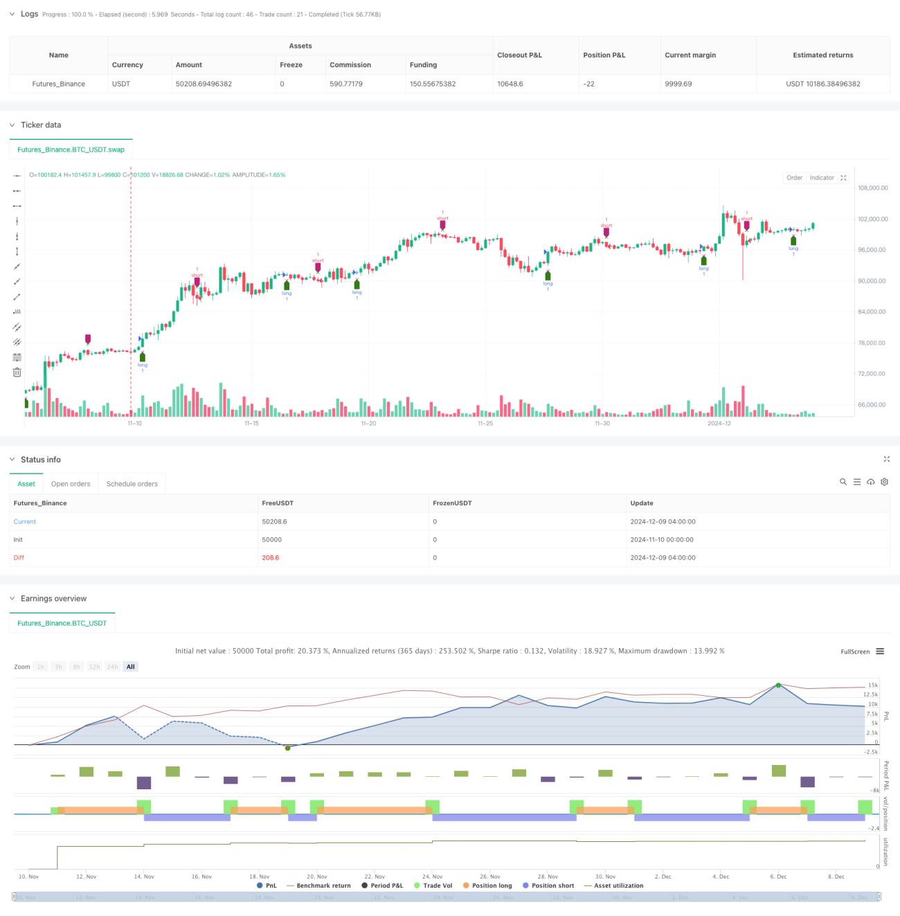
Code source de la stratégie
/*backtest
start: 2024-11-10 00:00:00
end: 2024-12-09 08:00:00
period: 4h
basePeriod: 4h
exchanges: [{"eid":"Futures_Binance","currency":"BTC_USDT"}]
*/

// This source code is subject to the terms of the Mozilla Public License 2.0 at https://mozilla.org/MPL/2.0/
// © tbiktag
//
// Delta-RSI Oscillator Strategy
//
// A strategy that uses Delta-RSI Oscillator (© tbiktag) as a stand-alone indicator:
// https://www.tradingview.com/script/OXQVFTQD-Delta-RSI-Oscillator/
//
// Delta-RSI is a smoothed time derivative of the RSI, plotted as a histogram 
// and serving as a momentum indicator. 
// 
// Input parameters:
// RSI Length: The timeframe of the RSI that serves as an input to D-RSI.
// Length: The length of the lookback frame used for local regression.
// Polynomial Order: The order of the local polynomial function used to interpolate the RSI.
// Signal Length: The length of a EMA of the D-RSI series that is used as a signal line.
// Trade signals are generated based on three optional conditions:
// - Zero-crossing: bullish when D-RSI crosses zero from negative to positive values (bearish otherwise)
// - Signal Line Crossing: bullish when D-RSI crosses from below to above the signal line (bearish otherwise)
// - Direction Change: bullish when D-RSI was negative and starts ascending (bearish otherwise)
//
// Since D-RSI oscillator is based on polynomial fitting of the RSI curve, there is also an option
// to filter trade signal by means of the root mean-square error of the fit (normalized by the sample average).
// 
//@version=5
strategy(title='Delta-RSI Oscillator Strategy-QuangVersion', shorttitle='D-RSI-Q', overlay=true)

// ---Subroutines---
matrix_get(_A, _i, _j, _nrows) =>
    // Get the value of the element of an implied 2d matrix
    //input: 
    // _A :: array: pseudo 2d matrix _A = [[column_0],[column_1],...,[column_(n-1)]]
    // _i :: integer: row number
    // _j :: integer: column number
    // _nrows :: integer: number of rows in the implied 2d matrix
    array.get(_A, _i + _nrows * _j)

matrix_set(_A, _value, _i, _j, _nrows) =>
    // Set a value to the element of an implied 2d matrix
    //input: 
    // _A :: array, changed on output: pseudo 2d matrix _A = [[column_0],[column_1],...,[column_(n-1)]]
    // _value :: float: the new value to be set
    // _i :: integer: row number
    // _j :: integer: column number
    // _nrows :: integer: number of rows in the implied 2d matrix
    array.set(_A, _i + _nrows * _j, _value)

transpose(_A, _nrows, _ncolumns) =>
    // Transpose an implied 2d matrix
    // input:
    // _A :: array: pseudo 2d matrix _A = [[column_0],[column_1],...,[column_(n-1)]]
    // _nrows :: integer: number of rows in _A
    // _ncolumns :: integer: number of columns in _A
    // output:
    // _AT :: array: pseudo 2d matrix with implied dimensions: _ncolums x _nrows
    var _AT = array.new_float(_nrows * _ncolumns, 0)
    for i = 0 to _nrows - 1 by 1
        for j = 0 to _ncolumns - 1 by 1
            matrix_set(_AT, matrix_get(_A, i, j, _nrows), j, i, _ncolumns)
    _AT

multiply(_A, _B, _nrowsA, _ncolumnsA, _ncolumnsB) =>
    // Calculate scalar product of two matrices
    // input: 
    // _A :: array: pseudo 2d matrix
    // _B :: array: pseudo 2d matrix
    // _nrowsA :: integer: number of rows in _A
    // _ncolumnsA :: integer: number of columns in _A
    // _ncolumnsB :: integer: number of columns in _B
    // output:
    // _C:: array: pseudo 2d matrix with implied dimensions _nrowsA x _ncolumnsB
    var _C = array.new_float(_nrowsA * _ncolumnsB, 0)
    int _nrowsB = _ncolumnsA
    float elementC = 0.0
    for i = 0 to _nrowsA - 1 by 1
        for j = 0 to _ncolumnsB - 1 by 1
            elementC := 0
            for k = 0 to _ncolumnsA - 1 by 1
                elementC += matrix_get(_A, i, k, _nrowsA) * matrix_get(_B, k, j, _nrowsB)
                elementC
            matrix_set(_C, elementC, i, j, _nrowsA)
    _C

vnorm(_X, _n) =>
    //Square norm of vector _X with size _n
    float _norm = 0.0
    for i = 0 to _n - 1 by 1
        _norm += math.pow(array.get(_X, i), 2)
        _norm
    math.sqrt(_norm)

qr_diag(_A, _nrows, _ncolumns) =>
    //QR Decomposition with Modified Gram-Schmidt Algorithm (Column-Oriented)
    // input:
    // _A :: array: pseudo 2d matrix _A = [[column_0],[column_1],...,[column_(n-1)]]
    // _nrows :: integer: number of rows in _A
    // _ncolumns :: integer: number of columns in _A
    // output:
    // _Q: unitary matrix, implied dimenstions _nrows x _ncolumns
    // _R: upper triangular matrix, implied dimansions _ncolumns x _ncolumns
    var _Q = array.new_float(_nrows * _ncolumns, 0)
    var _R = array.new_float(_ncolumns * _ncolumns, 0)
    var _a = array.new_float(_nrows, 0)
    var _q = array.new_float(_nrows, 0)
    float _r = 0.0
    float _aux = 0.0
    //get first column of _A and its norm:
    for i = 0 to _nrows - 1 by 1
        array.set(_a, i, matrix_get(_A, i, 0, _nrows))
    _r := vnorm(_a, _nrows)
    //assign first diagonal element of R and first column of Q
    matrix_set(_R, _r, 0, 0, _ncolumns)
    for i = 0 to _nrows - 1 by 1
        matrix_set(_Q, array.get(_a, i) / _r, i, 0, _nrows)
    if _ncolumns != 1
        //repeat for the rest of the columns
        for k = 1 to _ncolumns - 1 by 1
            for i = 0 to _nrows - 1 by 1
                array.set(_a, i, matrix_get(_A, i, k, _nrows))
            for j = 0 to k - 1 by 1
                //get R_jk as scalar product of Q_j column and A_k column:
                _r := 0
                for i = 0 to _nrows - 1 by 1
                    _r += matrix_get(_Q, i, j, _nrows) * array.get(_a, i)
                    _r
                matrix_set(_R, _r, j, k, _ncolumns)
                //update vector _a
                for i = 0 to _nrows - 1 by 1
                    _aux := array.get(_a, i) - _r * matrix_get(_Q, i, j, _nrows)
                    array.set(_a, i, _aux)
            //get diagonal R_kk and Q_k column
            _r := vnorm(_a, _nrows)
            matrix_set(_R, _r, k, k, _ncolumns)
            for i = 0 to _nrows - 1 by 1
                matrix_set(_Q, array.get(_a, i) / _r, i, k, _nrows)
    [_Q, _R]

pinv(_A, _nrows, _ncolumns) =>
    //Pseudoinverse of matrix _A calculated using QR decomposition
    // Input: 
    // _A:: array: implied as a (_nrows x _ncolumns) matrix _A = [[column_0],[column_1],...,[column_(_ncolumns-1)]]
    // Output: 
    // _Ainv:: array implied as a (_ncolumns x _nrows) matrix _A = [[row_0],[row_1],...,[row_(_nrows-1)]]
    // ----
    // First find the QR factorization of A: A = QR,
    // where R is upper triangular matrix.
    // Then _Ainv = R^-1*Q^T.
    // ----
    [_Q, _R] = qr_diag(_A, _nrows, _ncolumns)
    _QT = transpose(_Q, _nrows, _ncolumns)
    // Calculate Rinv:
    var _Rinv = array.new_float(_ncolumns * _ncolumns, 0)
    float _r = 0.0
    matrix_set(_Rinv, 1 / matrix_get(_R, 0, 0, _ncolumns), 0, 0, _ncolumns)
    if _ncolumns != 1
        for j = 1 to _ncolumns - 1 by 1
            for i = 0 to j - 1 by 1
                _r := 0.0
                for k = i to j - 1 by 1
                    _r += matrix_get(_Rinv, i, k, _ncolumns) * matrix_get(_R, k, j, _ncolumns)
                    _r
                matrix_set(_Rinv, _r, i, j, _ncolumns)
            for k = 0 to j - 1 by 1
                matrix_set(_Rinv, -matrix_get(_Rinv, k, j, _ncolumns) / matrix_get(_R, j, j, _ncolumns), k, j, _ncolumns)
            matrix_set(_Rinv, 1 / matrix_get(_R, j, j, _ncolumns), j, j, _ncolumns)
    //
    _Ainv = multiply(_Rinv, _QT, _ncolumns, _ncolumns, _nrows)
    _Ainv

norm_rmse(_x, _xhat) =>
    // Root Mean Square Error normalized to the sample mean
    // _x.   :: array float, original data
    // _xhat :: array float, model estimate
    // output
    // _nrmse:: float
    float _nrmse = 0.0
    if array.size(_x) != array.size(_xhat)
        _nrmse := na
        _nrmse
    else
        int _N = array.size(_x)
        float _mse = 0.0
        for i = 0 to _N - 1 by 1
            _mse += math.pow(array.get(_x, i) - array.get(_xhat, i), 2) / _N
            _mse
        _xmean = array.sum(_x) / _N
        _nrmse := math.sqrt(_mse) / _xmean
        _nrmse
    _nrmse


diff(_src, _window, _degree) =>
    // Polynomial differentiator
    // input:
    // _src:: input series
    // _window:: integer: wigth of the moving lookback window
    // _degree:: integer: degree of fitting polynomial
    // output:
    // _diff :: series: time derivative
    // _nrmse:: float: normalized root mean square error
    //
    // Vandermonde matrix with implied dimensions (window x degree+1)
    // Linear form: J = [ [z]^0, [z]^1, ... [z]^degree], with z = [ (1-window)/2 to (window-1)/2 ] 
    var _J = array.new_float(_window * (_degree + 1), 0)
    for i = 0 to _window - 1 by 1
        for j = 0 to _degree by 1
            matrix_set(_J, math.pow(i, j), i, j, _window)
    // Vector of raw datapoints:
    var _Y_raw = array.new_float(_window, na)
    for j = 0 to _window - 1 by 1
        array.set(_Y_raw, j, _src[_window - 1 - j])
    // Calculate polynomial coefficients which minimize the loss function
    _C = pinv(_J, _window, _degree + 1)
    _a_coef = multiply(_C, _Y_raw, _degree + 1, _window, 1)
    // For first derivative, approximate the last point (i.e. z=window-1) by 
    float _diff = 0.0
    for i = 1 to _degree by 1
        _diff += i * array.get(_a_coef, i) * math.pow(_window - 1, i - 1)
        _diff
    // Calculates data estimate (needed for rmse)
    _Y_hat = multiply(_J, _a_coef, _window, _degree + 1, 1)
    float _nrmse = norm_rmse(_Y_raw, _Y_hat)
    [_diff, _nrmse]

/// --- main ---
degree = input.int(title='Polynomial Order', group='Model Parameters:', inline='linepar1', defval=2, minval=1)
rsi_l = input.int(title='RSI Length', group='Model Parameters:', inline='linepar1', defval=21, minval=1, tooltip='The period length of RSI that is used as input.')
window = input.int(title='Length ( > Order)', group='Model Parameters:', inline='linepar2', defval=21, minval=2)
signalLength = input.int(title='Signal Length', group='Model Parameters:', inline='linepar2', defval=9, tooltip='The signal line is a EMA of the D-RSI time series.')
islong = input.bool(title='Buy', group='Show Signals:', inline='lineent', defval=true)
isshort = input.bool(title='Sell', group='Show Signals:', inline='lineent', defval=true)
showendlabels = input.bool(title='Exit', group='Show Signals:', inline='lineent', defval=true)
buycond = input.string(title='Buy', group='Entry and Exit Conditions:', inline='linecond', defval='Zero-Crossing', options=['Zero-Crossing', 'Signal Line Crossing', 'Direction Change'])
sellcond = input.string(title='Sell', group='Entry and Exit Conditions:', inline='linecond', defval='Zero-Crossing', options=['Zero-Crossing', 'Signal Line Crossing', 'Direction Change'])
endcond = input.string(title='Exit', group='Entry and Exit Conditions:', inline='linecond', defval='Zero-Crossing', options=['Zero-Crossing', 'Signal Line Crossing', 'Direction Change'])
usenrmse = input.bool(title='', group='Filter by Means of Root-Mean-Square Error of RSI Fitting:', inline='linermse', defval=false)
rmse_thrs = input.float(title='RSI fitting Error Threshold, %', group='Filter by Means of Root-Mean-Square Error of RSI Fitting:', inline='linermse', defval=10, minval=0.0) / 100


src = ta.rsi(close, rsi_l)
[drsi, nrmse] = diff(src, window, degree)
signalline = ta.ema(drsi, signalLength)

// Conditions and filters
filter_rmse = usenrmse ? nrmse < rmse_thrs : true
dirchangeup = drsi > drsi[1] and drsi[1] < drsi[2] and drsi[1] < 0.0
dirchangedw = drsi < drsi[1] and drsi[1] > drsi[2] and drsi[1] > 0.0
crossup = ta.crossover(drsi, 0.0)
crossdw = ta.crossunder(drsi, 0.0)
crosssignalup = ta.crossover(drsi, signalline)
crosssignaldw = ta.crossunder(drsi, signalline)

//Signals
golong = (buycond == 'Direction Change' ? dirchangeup : buycond == 'Zero-Crossing' ? crossup : crosssignalup) and filter_rmse
goshort = (sellcond == 'Direction Change' ? dirchangedw : sellcond == 'Zero-Crossing' ? crossdw : crosssignaldw) and filter_rmse
endlong = (endcond == 'Direction Change' ? dirchangedw : endcond == 'Zero-Crossing' ? crossdw : crosssignaldw) and filter_rmse
endshort = (endcond == 'Direction Change' ? dirchangeup : endcond == 'Zero-Crossing' ? crossup : crosssignalup) and filter_rmse
plotshape(golong and islong ? low : na, location=location.belowbar, style=shape.labelup, color=color.new(#2E7C13, 0), size=size.small, title='Buy')
plotshape(goshort and isshort ? high : na, location=location.abovebar, style=shape.labeldown, color=color.new(#BF217C, 0), size=size.small, title='Sell')
plotshape(showendlabels and endlong and islong ? high : na, location=location.abovebar, style=shape.xcross, color=color.new(#2E7C13, 0), size=size.tiny, title='Exit Long')
plotshape(showendlabels and endshort and isshort ? low : na, location=location.belowbar, style=shape.xcross, color=color.new(#BF217C, 0), size=size.tiny, title='Exit Short')

alertcondition(golong, title='Long Signal', message='D-RSI: Long Signal')
alertcondition(goshort, title='Short Signal', message='D-RSI: Short Signal')
alertcondition(endlong, title='Exit Long Signal', message='D-RSI: Exit Long')
alertcondition(endshort, title='Exit Short Signal', message='D-RSI: Exit Short')

strategy.entry('long', strategy.long, when=golong and islong)
strategy.entry('short', strategy.short, when=goshort and isshort)
strategy.close('long', when=endlong and islong)
strategy.close('short', when=endshort and isshort)