Stratégie de trading dynamique multidimensionnelle basée sur l'analyse du spectre quantique

Aperçu
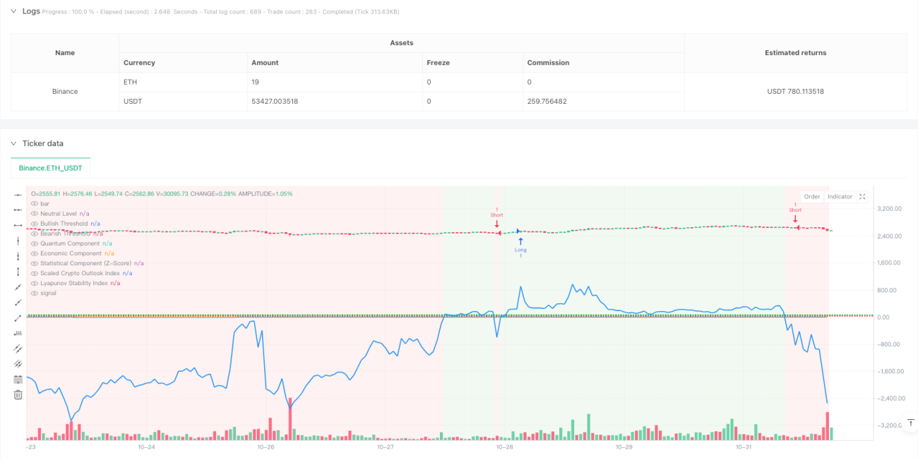
La stratégie est un système de trading quantifié innovant qui combine les principes de la mécanique quantique, de la statistique et de l'économie. Il construit un cadre d'analyse de marché complet en combinant des moyennes mobiles simples (SMA), des analyses statistiques de Z-Score, des composants de fluctuation quantique, des indicateurs de dynamique économique et de l'indice de stabilité de Lyapunov.
Principe de stratégie
La stratégie repose sur cinq piliers techniques principaux:
- Le module d'analyse statistique utilise le SMA et l'écart-type pour calculer le Z-Score, qui évalue la position relative des prix.
- Le composant quantique transforme le Z-Score en un oscillateur, qui simule les propriétés d'oscillation de l'état quantique par l'intermédiaire d'une fonction d'index et de résonance.
- La composante économique mesure la dynamique du marché en utilisant le rapport entre les EMA rapides et lents.
- L'indice de Lyapunov évalue l'état du marché en analysant la stabilité combinée des composants quantiques et économiques.
- L'indice global des perspectives de marché (COI) regroupe tous les composants de manière pondérée pour former le signal de négociation final.
Avantages stratégiques
- L'analyse multidimensionnelle fournit une vision plus globale du marché et réduit le biais qu'un seul indicateur peut entraîner.
- L'introduction de composants quantiques offre une perspective unique sur les fluctuations du marché, ce qui aide à saisir les opportunités à court terme.
- L'utilisation de l'indice Lyapunov permet d'évaluer efficacement la stabilité du marché et améliore la capacité de gestion des risques.
- La conception réglable en poids permet une adaptation flexible de la stratégie aux différentes conditions du marché.
- La conception de la ligne neutre de l'indice composite fournit une limite claire du signal de transaction.
Risque stratégique
- La multiplication des indicateurs peut entraîner un retard de signal et affecter le temps d'entrée.
- L'optimisation excessive des paramètres peut entraîner un risque de suradaptation.
- Les composants quantiques peuvent produire des signaux trop fréquents dans des marchés à forte volatilité.
- Les composants économiques peuvent générer des signaux trompeurs sur les marchés horizontaux.
- Il est nécessaire de mettre en place un stop-loss raisonnable pour contrôler les risques.
Orientation de l'optimisation de la stratégie
- La mise en place d'un système de poids adaptatif, permettant d'ajuster le poids des composants en fonction de l'évolution du marché.
- Augmentation du filtre de fréquence d'onde pour ajuster la sensibilité du signal pendant les hautes fréquences.
- L'intégration d'indicateurs de l'humeur du marché fournit des signaux de confirmation supplémentaires.
- Développer des mécanismes de stop-loss dynamiques afin d'adapter le niveau de stop-loss aux conditions du marché.
- Ajouter des filtres temporels pour éviter d'ouvrir une position à un moment défavorable.
Résumer
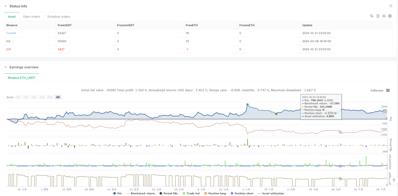
Il s'agit d'une stratégie de trading quantitatif innovante qui construit un cadre d'analyse de marché complet en fusionnant des théories multidisciplinaires. Bien qu'il y ait des points à optimiser, son approche d'analyse multidimensionnelle offre une perspective unique pour la prise de décision de trading. Grâce à l'amélioration continue de l'optimisation et de la gestion des risques, la stratégie devrait rester stable dans différents environnements de marché.
- 1